Assignment 1: A Matlab program for a 3D structure
Please refer the attached 2D frame program (Appendix A) with line-by-line explanations to develop a Matlab program for a 3D Frame, whose nodal and elemental information are shown in Appendix B. The shape of three types of cross section is given in Appendix C. The loading and boundary conditions are shown in Appendix D. Appendix E shows a schematic of frame element in 3D, the local stiffness matrix and material properties for the 3D structure. Noted that the gravity is not considered. In Appendix F, a sample Transmission tower is plotted and your program can be used directly for this complex structure. In Appendix G, analysis of 3D frame in Matlab is given via two examples.
The assignment should:
1) Write in terms of https://emedia.rmit.edu.au/learninglab/content/reports-0. A sample report is in Appendix B (10 point)
2) Introduce the theory of Finite Element Analysis for 3D frame. (10 point)
3) Plot the flow chart of the program. (10 point)
4) The structure is composed of 3 types of members. (15 point)
5) Plot the 3D Frame before deformation in a 3D view. The type of different members should be clearly seen in the figure. (15 point)
6) List the deformation of all nodes in a table. (20 point)
7) Write your understanding in Finite Element Analysis through this program. (10 point)
8) Please submit the report, Matlab program, input files (node.txt, elem.txt and etc.). (10 point)
Please upload the assignment to the blackboard before 00:00 19 Aug 2018. Late submissions will attract a penalty of 5% per day.
APPENDIX A
Finite element analysis for a 2D Frame in Matlab
|
Line |
Code |
explanation |
|
1 |
clc; |
Clear command window. |
|
2 |
clear; |
removes all variables from the workspace. |
|
3 |
close all; |
closes all the open figure windows. |
|
4 |
% blank line |
|
|
5 |
N = textread('node.txt'); |
Read x and y coordinate for the node and assign their values to N |
|
6 |
E = textread('elem.txt'); |
Read the near and far end for the beam and assign |
|
7 |
% blank line |
|
|
8 |
NN = length(N); |
Get the number of node |
|
9 |
NE = length(E); |
Get the number of element |
|
10 |
% blank line |
|
|
11 |
E0 = 2.1e6; |
Set Young’s modulus |
|
12 |
A0 = 22.8; |
Set the area of cross section |
|
13 |
I0 = 935; |
Set the second moment of inertia |
|
14 |
% blank line |
|
|
15 |
hold on; |
holds the current plot and all axis properties so that subsequent graphing commands add to the existing graph. |
|
16 |
for i=1:NE |
Begin an iteration in which i begins from 1 to NE |
|
17 |
plot([N(E(i,1),1),N(E(i,2),1)],[N(E(i,1),2),N( E(i,2),2)],'k','linewidth',2); |
Plot a line starts from the near end to the far end of an element in black with the linewidth of 2. |
|
18 |
text((N(E(i,1),1)+N(E(i,2),1))/2,(N(E(i,1),2)+ N(E(i,2),2))/2,num2str(i),'color','b','fontsiz e',12); |
Plot the element number at its middle in blue and 12 font size. |
|
19 |
end |
End the iteration |
|
20 |
% blank line |
|
|
21 |
for i=1:NN |
Begin an iteration in which i begins from 1 to NN |
|
22 |
if i<3 |
If i<3 |
|
23 |
plot(N(i,1),N(i,2),'rs','markersize',12,'mark erfacecolor','r'); |
Plot a red square marker at the node i with the size of 12 and red marker face color. |
|
24 |
else |
Else |
|
25 |
plot(N(i,1),N(i,2),'ko','markersize',8,'mark erfacecolor','k'); |
Plot a black circle marker at the node i with the size of 8 and black marker face color. |
|
26 |
end |
End if |
|
27 |
text(N(i,1),N(i,2),num2str(i),'color','g','font size',12); |
Plot a green node number at the node i with the size of 12. |
|
28 |
end |
End the iteration |
|
29 |
% blank line |
|
|
30 |
F=zeros(3*NN,1); |
Create the force vector and all members are zero. |
|
31 |
FN = [11 12 17 18 23 24]; |
Set the node number at which a load is applied |
|
32 |
F(3*FN-2) = -20; |
The x component of the load is -20 |
|
33 |
F(3*FN-1) = -10; |
The y component of the load is -10 |
|
34 |
% blank line |
|
|
35 |
scale = 20; |
Set the scaling factor |
|
36 |
for i=1:length(FN) |
Begin an iteration in which i begins from 1 to the number of loads |
|
37 |
plot( N(FN(i),1),N(FN(i),2),'b*','markersize' ,10,'markerfacecolor','b'); |
Plot a blue star with the size of 10 and blue marker face color at the node where a load is applied. |
|
38 |
plot([N(FN(i),1),N(FN(i),1)- 100*sin(20/180*pi)],[N(FN(i),2),N(FN(i),2) -100*cos(20/180*pi)],'- >r','linewidth',2,'markerfacecolor','r'); |
Plot red “>” symbols to show the applied load in 20 degree angle with line width of 2 and red marker face color |
|
39 |
% blank line |
|
|
40 |
ang=-1.5*pi:0.5:-.5*pi; |
|
|
41 |
xp=scale*cos(ang); |
|
|
42 |
yp=scale*sin(ang); |
|
|
43 |
plot(N(FN(i),1)+xp,N(FN(i),2)+yp,'– r>','linewidth',2,'markerfacecolor','r'); |
Plot 7 red “>” symbols to show the applied moment with line width of 2 and red marker face color |
|
44 |
end |
End the iteration |
|
45 |
% blank line |
|
|
46 |
title('A schematic of the power tower','fontsize',12); |
Plot the title of this figure with 12 font size |
|
47 |
set(gca,'fontsize',12); |
Set the font size of current axis as 12 |
|
48 |
axis equal tight |
Set the axis property as “equal” and “tight” |
|
49 |
print('-dtiff','-r400','frame.tif'); |
Print the figure in the name of “frame.tif” with tiff format and 400 resolution |
|
50 |
% blank line |
|
|
51 |
K=zeros(3*NN,3*NN); |
Determine the global stiffness matrix, its size is 3NN by 3NN and all members are zero. |
|
52 |
for n=1:NE |
Begin an iteration in which i begins from 1 to NN |
|
53 |
L = sqrt((N(E(n,1),1)-N(E(n,2),1))^2 + (N(E(n,1),2)-N(E(n,2),2))^2); |
Calculate the length of element |
|
54 |
lx = (N(E(n,2),1) – N(E(n,1),1))/L; |
Calculate cos(theta) |
|
55 |
ly = (N(E(n,2),2) – N(E(n,1),2))/L; |
Calculate sin(theta) |
|
56 |
a=A0*E0/L; |
Calculate some parameters for the local matrix |
|
57 |
b=6*E0*I0/L^2; |
Calculate some parameters for the local matrix |
|
58 |
c=12*E0*I0/L^3; |
Calculate some parameters for the local matrix |
|
59 |
d=E0*I0/L; |
Calculate some parameters for the local matrix |
|
60 |
% blank line |
|
|
61 |
Ke = [ a 0 0 -a 0 0 |
Determine the local matrix at local coordinate system |
|
62 |
0 c b 0 -c b |
|
|
63 |
0 b 4*d 0 -b 2*d |
|
|
64 |
-a 0 0 a 0 0 |
|
|
65 |
0 -c -b 0 c -b |
|
|
66 |
0 b 2*d 0 -b 4*d]; |
|
|
67 |
% blank line |
Determine the transformation matrix |
|
68 |
T = [ lx ly 0 0 0 0 |
|
|
69 |
-ly lx 0 0 0 0 |
|
|
70 |
0 0 1 0 0 0 |
|
71 |
0 0 0 lx ly 0 |
|
|
72 |
0 0 0 -ly lx 0 |
|
|
73 |
0 0 0 0 0 1]; |
|
|
74 |
% blank line |
|
|
75 |
Ke = T'*Ke*T; |
Determine the local matrix at global coordinate system |
|
76 |
i = E(n,1); |
Get the near end number of an element |
|
77 |
j = E(n,2); |
Get the far end number of an element |
|
78 |
dof = [3*i-2:3*i 3*j-2:3*j]; |
6 degrees of the element |
|
79 |
K(dof,dof) = K(dof,dof) + Ke; |
Assemble the global matrix from the local matrix |
|
80 |
end |
End the iteration |
|
81 |
% blank line |
|
|
82 |
fixeddofs = [1 2 3 4 5 6]; |
Fixed degrees |
|
83 |
alldofs = [1:3*NN]; |
All degrees |
|
84 |
freedofs = setdiff(alldofs,fixeddofs); |
Get the active degrees |
|
85 |
U(freedofs,:) = K(freedofs,freedofs)\F(freedofs,:); |
Calculate the equation Ax=b to get the deformations for all active degrees. |
|
86 |
U(fixeddofs,:)= 0; |
Make the fixed degrees equal zero |
|
87 |
% blank line |
|
|
88 |
figure; |
Plot a new figure |
|
89 |
hold on; |
holds the current plot and all axis properties so that subsequent graphing commands add to the existing graph. |
|
90 |
ND = N + scale*[U(1:3:end) U(2:3:end)]; |
Plot the node after the deformation. Noted the deformation is multiplied by the scaling factor. |
|
91 |
% blank line |
|
|
92 |
for i=1:NE |
Begin an iteration in which i begins from 1 to NN |
|
93 |
plot([N(E(i,1),1),N(E(i,2),1)],[N(E(i,1),2),N( E(i,2),2)],'linewidth',2,'color','k'); |
Plot a line starts from the near end (before deformation) to the far end (before deformation) of an element in black with the line width of 2. |
|
94 |
plot([ND(E(i,1),1),ND(E(i,2),1)],[ND(E(i,1),2 ),ND(E(i,2),2)],'–b','linewidth',2); |
Plot a line starts from the near end (after deformation)to the far end (after deformation) of an element in blue with the dashed line width of 2. |
|
95 |
end |
End the iteration |
|
96 |
% blank line |
|
|
97 |
title(['The deformation magnified ' int2str(scale) ' times'],'fontsize',12); |
Plot the title of this figure with 12 font size |
|
98 |
axis equal tight off |
Set the font size of current axis as 12 |
|
99 |
set(gca,'fontsize',12); |
Set the axis property as “equal” and “tight” |
|
100 |
print('-dtiff','-r400','U_frame.tif'); |
Print the figure in the name of “U_frame.tif” with tiff format and 400 resolution |
APPENDIX B
|
Node |
x |
y |
z |
|
1 |
-0.5 |
-0.3 |
0 |
|
2 |
0.5 |
-0.3 |
0 |
|
3 |
0.5 |
0.3 |
0 |
|
4 |
-0.5 |
0.3 |
0 |
|
5 6 7 8 |
-0.5 |
-0.3 |
2 |
|
0.5 |
-0.3 |
2 |
|
|
0.5 |
0.3 |
2 |
|
|
-0.5 |
0.3 |
2 |
|
Element number |
Element Type |
Final Node |
Initial Node |
|
1 |
1 |
1 |
5 |
|
2 |
1 |
2 |
6 |
|
3 |
1 |
3 |
7 |
|
4 |
1 |
4 |
8 |
|
5 |
2 |
5 |
6 |
|
6 |
2 |
6 |
7 |
|
7 |
2 |
7 |
8 |
|
8 |
2 |
8 |
5 |
|
9 |
3 |
1 |
6 |
|
10 |
3 |
2 |
7 |
|
11 |
3 |
3 |
8 |
|
12 |
3 |
4 |
5 |
APPENDIX C
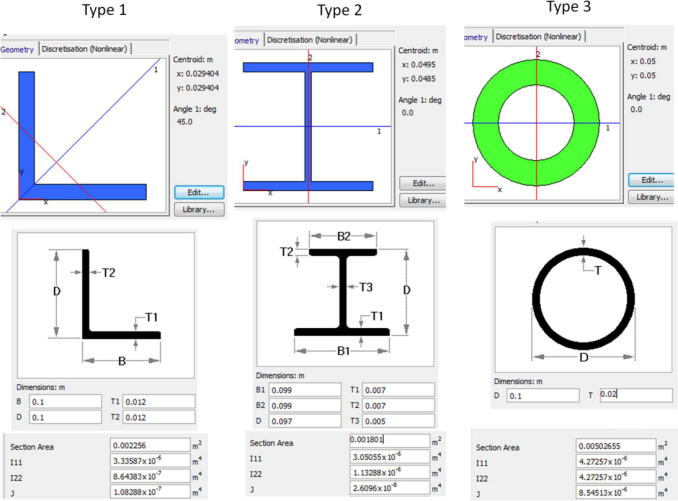
The cross section of three elements in the shape of Equal Angles, Welded Columns, and Circular Rings

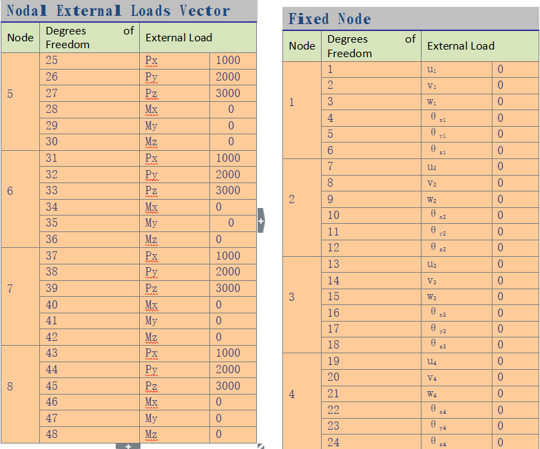
APPENDIX D

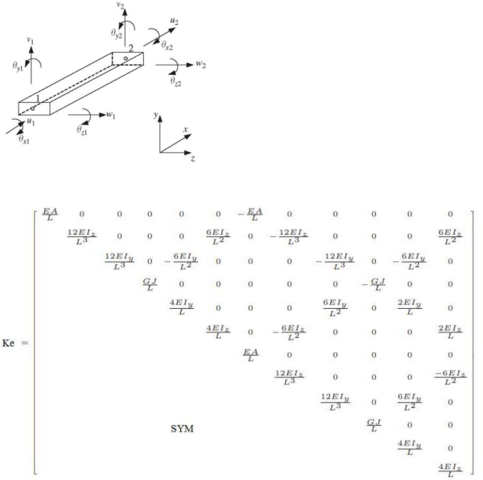
APPENDIX E:

Structural Steelwork (AS 4100-1998) pa Young’s modulus: E=2e11 pa
Shear Modulus: 8e10 pa
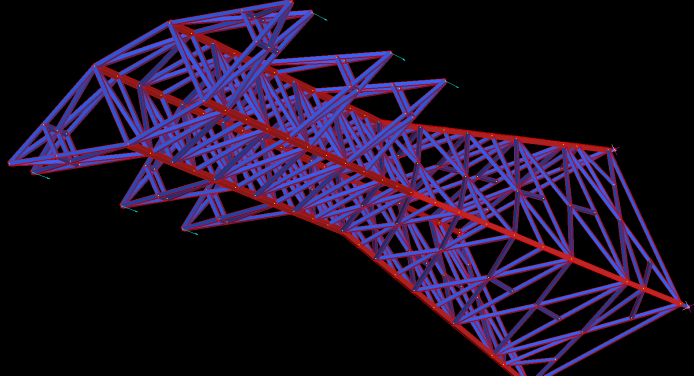
APPENDIX F: Sample Transmission tower

APPENDIX G: Finite Element Analysis of 3D Frame
代写CS&Finance|建模|代码|系统|报告|考试
编程类:C代写,JAVA代写 ,数据库代写,WEB代写,Python代写,Matlab代写,GO语言,R代写
金融类:统计,计量,风险投资,金融工程,R语言,Python语言,Matlab,建立模型,数据分析,数据处理
服务类:Lab/Assignment/Project/Course/Qzui/Midterm/Final/Exam/Test帮助代写代考辅导
天才写手,代写CS,代写finance,代写statistics,考试助攻
E-mail:[email protected] 微信:BadGeniuscs 工作时间:无休息工作日-早上8点到凌晨3点
如果您用的手机请先保存二维码到手机里面,识别图中二维码。如果用电脑,直接掏出手机果断扫描。

