
IAML – INFR10069 (LEVEL 10):
Assignment 2
python代写价格 We will employ tools for detecting misconduct. Moreover, please note that Piazza is NOT a forum for discussing the solutions of the assignment.
Due on Monday, 22 November, 2021 @ 16:00
NO LATE SUBMISSIONS
IMPORTANT INFORMATION
N.B. This document is best viewed on a screen as it contains a number of (highlighted) clickable hyperlinks.
It is very important that you read and follow the instructions below to the letter. You will be deducted marks for not adhering to the advice below.
Good Scholarly Practice: Please remember the University requirement regarding all assessed work for credit. Details about this can be found at: python代写价格
http://web.inf.ed.ac.uk/infweb/admin/policies/academic-misconduct
Specififically, this assignment should be your own individual work. We will employ tools for detecting misconduct. Moreover, please note that Piazza is NOT a forum for discussing the solutions of the assignment. You may, in exceptional circumstances, ask private questions to the instructors if you deem that something may be incorrect, and if we feel that the issue is justifified, we will send out an announcement.
General Instructions python代写价格
- There are two versions of this assignment. One for INFR10069 (level 10) and the other for INFR11182 (level 11). The level 11 version has some additional parts. MAKE SURE you are doing the assignment that corresponds to the course you are registered on;you can check this on EUCLID.
- We will use the IAML Learn page for any announcements, updates, and FAQs on this assign ment. Please visit the page frequently to fifind the latest information.
- You should use Python for implementing your solutions as this will standardise the output and also provide a consistent experience with the labs. If you are not using Notable, set up your environment as specifified in the Labs. It is VERY IMPORTANT that you use the exact same package versions as those specifified in the requirements fifile from the labs! Using the correct environment (i.e. py3iaml) is necessary to ensure that your outputs are consistent with the expected solutions. The correct package versions are specifified here.IAML – INFR10069 (LEVEL 10)
- If running import sklearn; print(sklearn.__version__) in your Jupyter Notebook does not print the package version 0.24.2, then you are not using the correct environment.
-
This assignment consists of multiple questions. MAKE SURE to use the correct dataset for each question.
- This assignment accounts for 30% of your fifinal grade for this course and is graded based on a written report (compiled from a latex template which we provide). You should submit not only the report, but also the code you wrote for the assignment. Since this is not a programming course, your code is not graded, but those answers in your report without corresponding code will not be graded.
- Some of the topics in this coursework are covered in weeks 7 and 8 of the course. Focus fifirst on questions on topics that you have covered already, and come back to the other questions as the lectures progress. python代写价格
- The criteria on which you will be judged include the quality of the textual answers and/or any plots asked for. For higher marks, when asked you need to give good and concise discussions based on experiments and theories using your own words.
- Read the instructions carefully, answering what is required and only that. Keep your answers brief and concise. Specififically, for textual answers, the size of the text-box in the latex template will give you an idea of the maximum length of your answer. You do not need to fifill in the whole text-box but you will be penalised if you go over. This does not apply to fifigure-based answers. python代写价格
- For answers involving fifigures, make sure to clearly label your plots and provide legends where necessary. You will be penalised if the visualisations are not clear.
- For answers involving numerical values, use correct units where appropriate and format flfloat ing point values to an appropriate number of decimal places.
Submission Mechanics
Important: You must submit this assignment by Monday, 22 November 2021 at 16:00. Extensions are not permitted and Extra Time Adjustments (ETA) for extensions are not permitted. For details, see the IAML coursework page on Learn.
- Your submission consists of a report (in PDF) and code. Marking is done based on the report submitted, whereas submitted code is mainly used to check your own individual work.
- We will use the Gradescope submission system for uploading report fifiles, and the Learn system for uploading code fifiles. Information describing how to upload your completed assignment will be made available on the IAML Learn page in Week 8.
- You should clone to your private repository or download the Assignment Repository from https://github.com/uoe-iaml/INFR10069-2021-CW2. python代写价格
This contains:
(a) The data you will need to complete the assignment under data directory.
(b) The helper function fifile under helpers directory, which you should use to load data in your program.
(c) The Python template fifiles under templates directory. They are iaml212cw2_q1.py,iaml212cw2_q2.py, and optionally iaml212cw2_my_helpers.py, which defifine the functions you should write in the assignment.
(d) Two tex fifiles, Assignment_2.tex and style.tex. These provide the template for you to fifill out the assignment questions. In particular, the template forces your answers to appear on separate pages and also controls the length of textual answers. python代写价格
-
You should modify the Assignment_2.tex template by:
(a) Uncommenting and specifying your student number at the top of the document (com pilation will automatically fail if you forget to do this). Remove the ‘%’ and enter your student number e.g.
\newcommand{\assignmentAuthorName}{s1234567}
(b) Filling in the answers in the provided answerbox environment. Note that some questions,e.g. Question 1.5, have multiple answerboxes spanning two pages.
DO NOT modify anything else in the template and certainly DO NOT edit the style fifile.
We reserve the right to not mark assignments which do not adhere to the template.
- Your should submit two fifiles of code, one for each of Questions 1 and 2, using the template fifiles specifified in the following table. Note that you should use the function names specifified in the templates for each question. You should not change the function names or fifile names. In case you use helper functions of your own, you should also submit them as a single fifile with the fifile name specifified in the table. Jupyter Notebook fifiles (.ipynb) can be submitted instead of Python (.py) fifiles. If it is the case, you should replace “.py” with “.ipynb”. In Jupyter fifiles, you do not need to use the specifified functions, but you should indicate the function names as comments in the corresponding cells.
Latex Tips python代写价格
- To fifill in text answers, you can modify the text inside the answerbox:
\ begi n { answerbox }{5em}
Your answer h e r e
\ end{ answerbox }
with your answer (replacing ‘Your answer here’):
\ begi n { answerbox }{5em}
Steam l o c om o ti v e s were f i r s t de veloped i n the United Kingdom
du ring the e a r l y 19 th c e n t u r y and used f o r r ail w a y t r a n s p o r t
u n t i l the middle of the 20 th c e n t u r y .
\ end{ answerbox }
which, when compiled gives: python代写价格
Steam locomotives were fifirst developed in the United Kingdom during the early 19th century and used for railway transport until the middle of the 20th century.
-
To add an image, you can use:
\ begi n { answerbox }{18em}
This image shows a t r a i n .
\ begi n { c e n t e r }
\ i n c l u d e g r a p h i c s [ width =0.6\ t e x twi d t h ] { stock_image . jpg }
\ end{ c e n t e r }
\ end{ answerbox }
which will be compiled to:
This image shows a train.
Make sure that you specify the correct path to your image. For example. if your image was stored in a directory called results, you would change the relevant line to read:
\ i n c l u d e g r a p h i c s [ width =0.6\ t e x twi d t h ] { r e s u l t s / stock_image . jpg } python代写价格
You can fifind more information about inserting images into latex documents here.
- You can also add two images side-by-side:
\ begi n { answerbox }{18em}
Below we s e e two t r a i n s .
\ begi n { c e n t e r }
\ begi n { t a b ul a r }{ l l }
\ i n c l u d e g r a p h i c s [ width =0.4\ t e x twi d t h ] { stock_image . jpg }
&
\ i n c l u d e g r a p h i c s [ width =0.4\ t e x twi d t h ] { stock_image . jpg }
\ end{ t a b ul a r }
\ end{ c e n t e r }
\ end{ answerbox }
which will be compiled to:
Below we see two trains.
-
To add an inline equation, you can use the ‘$’ symbol to write:
\ begi n { answerbox }{3em}
I am u si ng the f o l l o w i n g model , $y = \mathbf{x}^T\mathbf{w}$ .
\ end{ answerbox }
which compiles to:
I am using the following model, y = xT w.
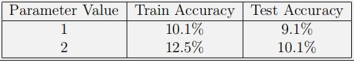
- To add a table for numerical results you can use:
\ begi n { answerbox }{7em}
R e s ul t s a r e p r e s e n t e d i n the t a b l e below .
\ begi n { c e n t e r }
\ begi n { t a b ul a r }{ | c | c | c | } \ h l i n e
Parameter Value & Train Accuracy & Test Accuracy \\ \ h l i n e
1 & 10.1\% & 9.1\% \\
2 & 12.5\% & 10.1\% \\\ h l i n e
\ end{ t a b ul a r }
\ end{ c e n t e r }
\ end{ answerbox }
which compiles to:
Results are presented in the table below.
You can fifind more information about tables in latex here.
- For a small number of questions we may ask you to show your code in your report. You can include code as an image, but if you prefer you can use the following command:
\ begi n { answerbox }{5em}
\ begi n { ve rba tim }
import numpy a s np
mean_time = 10.0
p r i n t ( `mean time ‘ , mean_time )
\ end{ ve rba tim }
\ end{ answerbox }
which, when compiled gives:
import numpy as np
mean_time = 10.0
print(‘mean time’, mean_time)
- Once you have fifilled in all the answers, compile the latex document to generate the PDF that you will submit. You can use Overleaf, your favourite latex editor, or just run pdflatex Assignment_2.tex twice on a DICE machine to compile the PDF. python代写价格

Question 1 : (70 total points) Experiments on a binary-classifification data set
In this question we look into basic techniques for data analysis and classifification using a data set for binary classifification.
The data set is a collection of medical records of 800 people, where each record consists of nine real-valued features, which are the measurements for attributes ’A0’,. . .,’A8’, and a binary class label of 0 or 1, where 1 indicates that the person has a particular disease, and 0 indicates that they do not. Load the data set and apply some processing in the following manner in your code.
import s ci p y
import numpy a s np
from iaml_cw2_helpers import ∗
X, Y = load_Q1_dataset ( )
p r i n t ( ‘X: ‘ , X. shape , ‘Y: ‘ , Y. shape )
Xtrn = X[ 1 0 0 : , : ] ; Ytrn = Y[ 1 0 0 : ] # t r a i n i n g data s e t
Xtst = X[ 0 : 1 0 0 , : ] ; Ytst = Y[ 0 : 1 0 0 ] # t e s t data s e t
Make sure that X is a 800-by-9 array and Y is a vector of 800 elements. X holds the features and Y holds labels. { Xtrn, Ytrn } is a training set, and { Xtst, Ytst } a test set, Note that you should NOT shufflfflffle the data. python代写价格
1.1 (9 points)
We want to see how each feature in Xtrn is distributed for each class. Since there are nine attributes, we plot a total of nine fifigures in a 3-by-3 grid, where the top-left fifigure shows the histograms for attribute ’A0’ and the bottom-right ’A8’. In each fifigure, you show histograms of instances of class 0 and those of class 1 using pyplot.hist([Xa, Xb], bins=15), where Xa corresponds to instances of class 0 and Xb to those of class 1, and you set the number of bins to 15.Use grid lines. Based on the results you obtain, discuss and explain your fifindings.
1.2(9 points)
Calculate the correlation coeffiffifficient between each attribute of Xtrn and the label Ytrn, so that you calculate nine correlation coeffiffifficients. Answer the following questions.
(a) Report the correlation coeffiffifficients in a table.
(b) Discuss if it is a good idea to use the attributes that have large correlations with the label for classifification tasks.
(c) Discuss if it is a good idea to ignore the attributes that have small correlations with the label for classifification tasks. python代写价格
1.3 (4 points)
We consider a set of instances of two variables, {(ui , vi)} N i=1, where N denotes the number of instances. Show (using your own words and mathematical expressions) that the correla tion coeffiffifficient between the two variables, ruv, is translation invariant and scale invariant, i.e. ruv does not change under linear transformation, a + bui and c + dvi for i = 1, . . . , N, where a, b, c, d are constants and b > 0, d > 0.
1.4 (5 points) Calculate the unbiased sample variance of each attribute of Xtrn, and sort the variances in decreasing order. Answer the following questions.
(a) Report the sum of all the variances.
(b) Plot the following two graphs side-by-side. Use grid lines in each plot.
- A graph of the amount of variance explained by each of the (sorted) attributes, where you indicate attribute numbers on the x-axis.
- A graph of the cumulative variance ratio against the number of attributes, where the range of y-axis should be [0, 1].
1.5 (8 points) python代写价格
Apply Principal Component Analysis (PCA) to Xtrn, where you should not rescale Xtrn. Use Sklearn’s PCA with default parameters, i.e. specifying no parameters.
(a) Report the total amount of unbiased sample variance explained by the whole set of principal components.
(b) Plot the following two graphs side-by-side. Use grid lines in each plot.
- A graph of the amount of variance explained by each of the principal components.
- A graph of the cumulative variance ratio, where the range of y-axis should be [0, 1].
(c) Mapping all the instances in Xtrn on to the 2D space spanned with the fifirst two principal components, and plot a scatter graph of the instances on the space, where instances of class 0 are displayed in blue and those of class 1 in red. Use grid lines. Note that the mapping should be done directly using the eigen vectors obtained in PCA – you should not use Sklearn’s functions, e.g. transform().
(d) Calculate the correlation coeffiffifficient between each attribute and each of the fifirst and second principal components, report the result in a table.
1.6 (4 points)
We now standardise the data by mean and standard deviation using the method described below, and look into how the standardisation has impacts on PCA. Create the standardised training data Xtrn_s and test data Xtst_s in your code in the following manner.
from s k l e a r n . p r e p r o c e s s i n g import S ta n da r d S cal e r
s c a l e r = S ta n da r d S cal e r ( ) . f i t ( Xtrn )
Xtrn_s = s c a l e r . t ra n sfo rm ( Xtrn ) # s t a n d a r di s e d t r a i n i n g data
Xtst_s = s c a l e r . t ra n sfo rm ( Xtst ) # s t a n d a r di s e d t e s t data
Using the standardised data Xtrn_s instead of Xtrn, answer the questions (a), (b), (c), and (d) in1.5.
1.7 (7 points) Based on the results you obtained in 1.4, 1.5, and 1.6, answer the following questions.
(a) Comparing the results of 1.4 and 1.5, discuss and explain your fifindings. python代写价格
(b) Comparing the results of 1.5 and 1.6, discuss and explain your fifindings and discuss (using your own words) whether you are strongly advised to standardise this particular data set beforePCA.
1.8 (12 points)
We now want to run experiments on Support Vector Machines (SVMs) with a RBF kernel, where we try to optimise the penalty parameter C. By using 5-fold CV on the standardised training data Xtrn_s described above, estimate the classifification accuracy, while you vary the penalty parameter C in the range 0.01 to 100 – use 13 values spaced equally in log space, where the logarithm base is 10. Use Sklearn’s SVC and StratifiedKFold with default parameters unless specifified. Do not shufflfflffle the data.
Answer the following questions.
(a) Calculate the mean and standard deviation of cross-validation classifification accuracy for each C, and plot them against C by using a log-scale for the x-axis, where standard deviations are shown with error bars. On the same fifigure, plot the same information (i.e. the mean and standard deviation of classifification accuracy) for the training set in the cross validation.
(b) Comment (in brief) on any observations.
(c) Report the highest mean cross-validation accuracy and the value of C which yielded it.
(d) Using the best parameter value you found, evaluate the corresponding best classififier on the test set { Xtst_s, Ytst }. Report the number of instances correctly classifified and classifification accuracy.
1.9 (5 points)
We here consider a two-dimensional (2D) Gaussian distribution for a set of two dimensional vectors, which we form by selecting a pair of attributes, A4 and A7, in Xtrn (NB: not Xtrn_s) whose label is 0. To make the distribution of data simpler, we ignore the instances whose A4 value is less than 1. Save the resultant set of 2D vectors to a Numpy array, Ztrn, where the fifirst dimension corresponds to A4 and the second to A7. You will fifind 318 instances in Ztrn. python代写价格
Using Numpy’s libraries, estimate the sample mean vector and unbiased sample covariance matrix of a 2D Gaussian distribution for Ztrn. Answer the following questions.
(a) Report the mean vector and covariance matrix of the Gaussian distribution.
(b) Make a scatter plot of the instances and display the contours of the estimated distribution on it using Matplotlib’s contour. Note that the fifirst dimension of Ztrn should correspnd to the x-axis and the second to y-axis. Use the same scaling (i.e. equal aspect) for the x-axis and y-axis, and show grid lines.
1.10 (7 points)
Assuming naive-Bayes, estimate the model parameters of a 2D Gaussian distribution for the data Ztrn you created in 1.9, and answer the following questions.
(a) Report the sample mean vector and unbiased sample covariance matrix of the Gaussian dis tribution.
(b) Make a new scatter plot of the instances in Ztrn and display the contours of the estimated distribution on it. Note that you should always correspond the fifirst dimension of Ztrn to x-axis and the second dimension to y-axis. Use the same scaling (i.e. equal aspect) for x-axis and y-axis, and show grid lines.
(c) Comparing the result with the one you obtained in 1.9, discuss and explain your fifindings, and discuss if it is a good idea to employ the naive Bayes assumption for this data Ztrn. python代写价格
Question 2 : (75 total points) Experiments on an image data set of handwritten letters
Image data are made up of H × W × C pixels, where H, W, C denote the height, width, and the number of channels, respectively. For simplicity, we assume a grayscale image (i.e. C=1). Let pij denote the pixel value at a grid point (i, j), 1 ≤ i ≤ H, 1 ≤ j ≤ W, where p11 corresponds to the the pixel at the top-left corner and pHW to the one at the bottom-right corner. We assume that pij takes an integer value between 0 and 255 (i.e. 8-bit coding). In computers, we can store a grayscale image of {pij} in a D-dimensional vector, x = (x1, x2, . . . , xD), where D = H × W, and x1 corresponds to p11 and xD to pHW .
Here we use a subset of the EMNIST data set of images, restricting characters to the English alphabet of 26 letters in upper case. The class labels are given in alphabetical order, where class 0 corresponds to ’A’ and 25 to ’Z’. There are 300 training instances and 100 test instances per class.
Each instance is a 28-by-28 grayscale image. Note that you will fifind some errors (e.g. incorrect labels) in the data set, but we use the data set as it is.
Load the data and apply some pre-processing in the following manner in your code.
import s ci p y
import numpy a s np
from iaml_cw2_helpers import ∗
Xtrn_org , Ytrn_org , Xtst_org , Ytst_org = load_Q2_dataset ( )
Xtrn = Xtrn_org / 255.0
Xtst = Xtst_org / 255.0
Ytrn = Ytrn_org − 1
Ytst = Ytst_org − 1
Xmean = np . mean ( Xtrn , a x i s =0)
Xtrn_m = Xtrn − Xmean ; Xtst_m = Xtst − Xmean # Mean−no rmali s e d v e r s i o n s
where { Xtrn, Ytrn } is the training set (Xtrn holds instances of images and Ytrn holds correspond ing labels), { Xtst, Ytst } is the test set, and Xtrn_m and Xtst_m are the mean-subtracted versions of Xtrn and Xtst, respectively. You should NOT change the order or apply any transformation to the data unless specifified.
2.1 (5 points) python代写价格
(a) Report (using a table) the minimum, maximum, mean, and standard deviation of pixel values for each Xtrn and Xtst. (Note that we mean a single value of each of min, max, etc. for each Xtrn and Xtst.)
(b) Display the gray-scale images of the fifirst two instances in Xtrn properly, clarifying the class number for each image. The background colour should be white and the foreground colour black. python代写价格
2.2 (4 points)
(a) Xtrn_m is a mean-vector subtracted version of Xtrn. Discuss if the Euclidean distance between a pair of instances in Xtrn_m is the same as that in Xtrn.
(b) Xtst_m is a mean-vector subtracted version of Xtst, where the mean vector of Xtrn was employed in the subtraction instead of the one of Xtst. Discuss whether we should instead use the mean vector of Xtst in the subtraction.
2.3 (7 points)
Apply k-means clustering to the instances of each of class 0, 5, 8 (i.e. ’A’, ’F’, ’I’) in Xtrn with k = 3, 5, for which use Sklearn’s KMeans with n_clusters=k and random_state=0 while using default values for the other parameters. Note that you should apply the clustering to each class separately. Make sure you use Xtrn rather than Xtrn_m. Answer the following questions.
(a) Display the images of cluster centres for each k, so that you show two plots, one for k = 3 and the other for k = 5. Each plot displays the grayscale images of cluster centres in a 3-by-k grid, where each row corresponds to a class and each column to cluster number, so that the top-left grid item corresponds to class 0 and the fifirst cluster, and the bottom-right one to class 8 and the last cluster.
(b) Discuss and explain your fifindings, including discussions if there are any concerns of using this data set for classifification tasks.
2.4 (5 points) Explain (using your own words) why the sum of square error (SSE) in k-means clustering does not increase for each of the following cases.
(a) Clustering with k + 1 clusters compared with clustering with k clusters.
(b) The update step at time t + 1 compared with the update step at time t when clustering with k clusters.
2.5 (11 points)
Here we apply multi-class logistic regression classifification to the data. You should use Sklearn’s LogisticRegression with parameters ’max_iter=1000’ and ’random_state=0’ while use default values for the other parameters. Use Xtrn_m for training and Xtst_m for testing. We do not employ cross validation here. Carry out a classifification experiment.
(a) Report the classifification accuracy for each of the training set and test set.
(b) Find the top fifive classes that were misclassifified most in the test set. You should provide the class numbers, corresponding alphabet letters (e.g. A,B,. . .), and the numbers of misclassififi-cations.
(c) For each class that you identifified in the above, make a quick investigation and explain possiblereasons for the misclassififications. python代写价格
2.6 (20 points) Without changing the learning algorithm (i.e. use logistic regression), your task here is to improve the classifification performance of the model in 2.5. Any training and optimisation(e.g. hyper parameter tuning) should be done within the training set only. Answer the following questions.
(a) Discuss (using your own wards) three possible approaches to improve classifification accuracy,decide which one(s) to implement, and report your choice.
(b) Brieflfly describe your implemented approach/algorithm so that other people can understand it without seeing your code. If any optimisation (e.g. parameter searching) is involved, clarify and describe how it was done.
(c) Carry out experiments using the new classifification system, and report the results, including results of parameter optimisation (if any) and classifification accuracy for the test set. Comments on the results.
2.7 (9 points) python代写价格
Using the training data of class 0 (’A’) from the training set Xtrn_m, calculate the sample mean vector, and unbiased sample covariance matrix using Numpy’s functions, and answer the following.
(a) Report the minimum, maximum, and mean values of the elements of the covariance matrix.
(b) Report the minimum, maximum, and mean values of the diagonal elements of the covariance matrix.
(c) Show the histogram of the diagonal values of the covariance matrix. Set the number of bins to 15, and use grid lines in your plot.
(d) Using Scipy’s multivariate_normal with the mean vector and covariance matrix you ob tained, try calculating the likelihood of the fifirst element of class 0 in the test set (Xtst_m).You will receive an error message. Report the main part of error message, i.e. the last line of the message, and explain why you received the error, clarifying the problem with the data you used.
(e) Discuss (using your own words) three possible options you would employ to avoid the error.
Note that your answer should not include using a difffferent data set.
2.8 (8 marks)
Instead of Scipy’s multivariate_normal we used in 2.7, we now use Sklearn’s GaussianMixture with parameters, n_components=1, covariance_type=’full’, so that there is a single Gaussian distribution fifitted to the data. Use { Xtrn_m, Ytrn } as the training set and {Xtst_m, Ytst } as the test set.
(a) Train the model using the data of class 0 (’A’) in the training set, and report the log-likelihood of the fifirst instance in the test set with the model. Explain why you could calculate the value this time.
(b) We now carry out a classifification experiment considering all the 26 classes, for which we assign a separate Gaussian distribution to each class. Train the model for each class on the training set, run a classifification experiment using a multivariate Gaussian classififier, and report the number of correctly classifified instances and classifification accuracy for each training set andtest set. python代写价格
(c) Brieflfly comment on the result you obtained.
2.9 (6 points) Answer the following question on Gaussian Mixture Models (GMMs).
(a) Explain (using your own words) why Maximum Likelihood Estimation (MLE) cannot be applied to the training of GMMs directly.
(b) The Expectation Maximisation (EM) algorithm is normally used for the training of GMMs,but another training algorithm is possible, in which you employ k-means clustering to split the training data into clusters and apply MLE to estimate model parameters of a Gaussian distribution for each cluster. Explain the difffference between the two algorithms in terms of parameter estimation of GMMs.