AUGUST 2018 EXAMINATION DIET SCHOOL OF MATHEMATICS & STATISTICS
统计推断代考 LetX1, . . . , Xn denote the lifetime of a particular brand of The manu- facturer guarantees that the mean useful lifetime of a tyre is 42500 miles.
MODULE CODE: MT2508
MODULE TITLE: Statistical Inference
EXAM DURATION: 2 hours
EXAM INSTRUCTIONS: Attempt ALL questions.
The number in square brackets shows the maximum marks obtainable for that question or part-question.
Your answers should contain the full working required to justify your solutions.
PERMITTED MATERIALS: Non-programmable calculator
YOU MUST HAND IN THIS EXAM PAPER AT THE END OF THE EXAM
PLEASE DO NOT TURN OVER THIS EXAM PAPER UNTIL YOU ARE INSTRUCTED TO DO SO.
1.LetX1, . . . , Xn denote independent and identically distributed normal random variables such that Xi ∼ N (µ, σ2) for i = 1, . . . , n, where σ2 is unknown. 统计推断代考
(a)Determine whether or not the following statements are true or false. Jus- tify your answers.
(i)Thesample mean X¯is an unbiased and consistent estimator of µ. [2]
(ii)X1Xnis an unbiased estimator of µ2. [2]
(iii)X¯ − X1 + Xn is an unbiased estimator of µ. [2]
(iv)X¯ − X1 + Xn is a consistent estimator of µ. [3]
(b)Statethe distribution of Y = Σn Xi. [1]
(c)Hence, derive a 100(1 − α)% confidence interval for nµ. [5]
You may use the following results without proof:
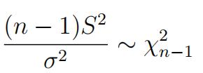
S2 and¯X are independent.
2.LetY1, . . . , Yn denote independent random variables such that Yi ∼ N (µi, σ2) for i = 1, . . . , n. Consider the case µi = αxi where α is an unknown parameter and x1, . . . , xn are known observations.
(a)Showthat the likelihood function for observations y1, . . . , yn is given by,
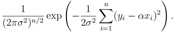
[2]
(b)Showthat the maximum likelihood estimator for α is given by,
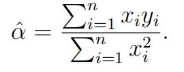 [3]
[3]
(c)Derive the maximum likelihood estimatorfor σ2. [3]
(d)Hence, state the maximum likelihood estimator for σ. Justify your answer.[2]
3.LetX1, . . . , Xn denote the lifetime of a particular brand of The manu- facturer guarantees that the mean useful lifetime of a tyre is 42500 miles. 统计推断代考
A consumer test agency has received complaints that the mean lifetime of the tyre is less than that guaranteed. Wishing to test the manufacturer’s claim, the test agency observed 10 tyres on a test wheel that simulated normal road conditions. The lifetimes (in thousands of miles) were as follows:
41 35 45 42 40 34 42 40 39 38
(a)State appropriate null and alternative hypotheses for testing whether or notthe mean lifetime of the tyre is as the manufacturer has Define any notation you use. [2]
(b)State the name of a parametric test that could be used to test the hy- potheses in part (a). State the assumptions of yourchosen test. [3]
(c)Perform the test chosen in part (b) at the 1% level by finding thep-value
of the test. Clearly state your conclusions. [5] 统计推断代考
The following R output may be useful.
> pnorm(-2.77) [1] 0.002802815
> qnorm(0.84) [1] 0.9944579
> 1-pt(2.77, 9)
[1] 0.01087675> 1-pt(0.84, 9)
[1] 0.2113305(d)Calculate a 99% confidence interval for the mean lifetime of a tyre of this brand. [2]
The following R output may be useful.
> pt(0.005, 9)
[1] 0.5019402> qt(0.995, 9)
[1] 3.249836> qnorm(0.995) [1] 2.575829
> pnorm(-1.96) [1] 0.0249979
(e)Does your confidence interval from part (d) agree with the result of the hypothesis test from part (c)? Justifyyour [2]

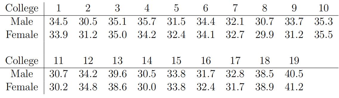
4.The following table shows data on average salaries ($1000/yr) for male and female assistant professors at 19 US colleges, selected at random. 统计推断代考
 Consider the following R session.
1: > dataM <- c(34.5, 30.5, 35.1, 35.7, 31.5, 34.4, 32.1, 30.7,

+ 33.7, 35.3, 30.7, 34.2, 39.6, 30.5, 33.8, 31.7,

+ 32.8, 38.5, 40.5)

2: > dataF <- c(33.9, 31.2, 35.0, 34.2, 32.4, 34.1, 32.7, 29.9,

+ 31.2, 35.5, 30.2, 34.8, 38.6, 30.0, 33.8, 32.4,

+ 31.7, 38.9, 41.2)

3: > diff <- dataM - dataF

> diff

[1] 0.6 -0.7 0.1 1.5 -0.9 0.3 -0.6 0.8 2.5 -0.2

[11] 0.5 -0.6 1.0 0.5 0.0 -0.7 1.1 -0.4 -0.7

4: > wilcox.test(dataM[diff != 0], dataF[diff != 0], paired=T)

Wilcoxon signed rank test with continuity correction

data: dataM[diff != 0] and dataF[diff != 0]

V = 102.5, p-value = 0.4722

alternative hypothesis: true location shift is not equal to 0

Warning message:

In wilcox.test.default(dataM[diff != 0], dataF[diff != 0], paired = T) :

cannot compute exact p-value with ties

5: > mystery.function <- function(num, data) {

6: + res <- rep(0, num+1)

7: + for (i in 1:num) {

8: + sign <- sample(c(-1,1), length(data), replace=T)

9: + rand <- data*sign

10: + res[i] <- mean(rand)

+ }

11: + res[num+1] <- mean(data)

12: + f <- sum(res >= mean(data))

13: + if (f <= ((num+1)/2)) {

14: + p <- 2*(f/(num+1))

15: + } else {

16: + p <- 2*(1-(f/(num+1)))

+ }

17: + p

+ }

18: > mystery.function(999, diff[diff != 0])

[1] 0.346
(a)Explain what each of the numbered lines of code in the above R session is doing.[5]
(b)State the name of the test being performed by mystery.function.[1]
(c)State the defifinitions of a p-value and a Type I error.[2] 统计推断代考
(d)Do these data provide evidence of discrimination? Justify your answer.[2]
(e)Explain why the p-values from the two analyses above are difffferent. Which test is more powerful?[2]
(f)Calculate the p-value for a sign test where the alternative hypothesis is two-sided.[2]
The following R output may be useful.
> 1-pbinom(9,18,0.5)

[1] 0.4072647

> 1-pbinom(10,18,0.5)

[1] 0.2403412

> 1-pbinom(9,19,0.5)

[1] 0.5

> 1-pbinom(10,19,0.5)

[1] 0.3238029
(g)Explain how a randomisation test diffffers from a permutation test. Give one advantage of each method.
5.For a certain module with 68 students, the lecturer models the relationship of thestudents’ final exam mark (as a percentage) as a linear function of the asso- ciated marks on two practical assignments and a class test. 统计推断代考
The students’ exam marks are stored in the vector exam and the associated coursework marks are in vectors prac1, prac2 and classtest. The following analysis is conducted in R.
> exammod1 <- lm(exam ~ classtest + prac1 + prac2)
> summary(exammod1)
Call:
lm(formula = exam ~ classtest + prac1 + prac2)
Residuals:
Min 1Q Median 3Q Max
-7.7601 -1.6476 -0.3917 2.1157 10.3303
Coefficients:
Estimate Std. Error t value Pr(>|t|) (Intercept) -5.9330 1.1655 -5.090 3.37e-06 ***
classtest 0.3497 0.2805 1.247 0.217029
prac1 0.5516 0.4476 1.232 0.222322
prac2 0.7925 0.2008 3.948 0.000199 ***
—
Signif. codes: 0 *** 0.001 ** 0.01 * 0.05 . 0.1 1
Residual standard error: 3.594 on 64 degrees of freedom Multiple R-squared: 0.98,Adjusted R-squared: 0.979
F-statistic: 1044 on 3 and 64 DF, p-value: < 2.2e-16
> exammod2 <- lm(exam ~ classtest + prac2)
> summary(exammod2)
Call:
lm(formula = exam ~ classtest + prac2) 统计推断代考
Residuals:
Min 1Q Median 3Q Max
-8.7876 -1.5966 -0.3051 2.0557 10.7195
Coefficients:
Estimate Std. Error t value Pr(>|t|) (Intercept) -5.7816 1.1636 -4.969 5.18e-06 ***
classtest 0.6670 0.1119 5.963 1.12e-07 ***
prac2 0.8968 0.1828 4.907 6.51e-06 ***
—
Signif. codes: 0 *** 0.001 ** 0.01 * 0.05 . 0.1 1
Residual standard error: 3.608 on 65 degrees of freedom
Multiple R-squared: 0.9795,Adjusted R-squared: 0.9789
F-statistic: 1552 on 2 and 65 DF, p-value: < 2.2e-16
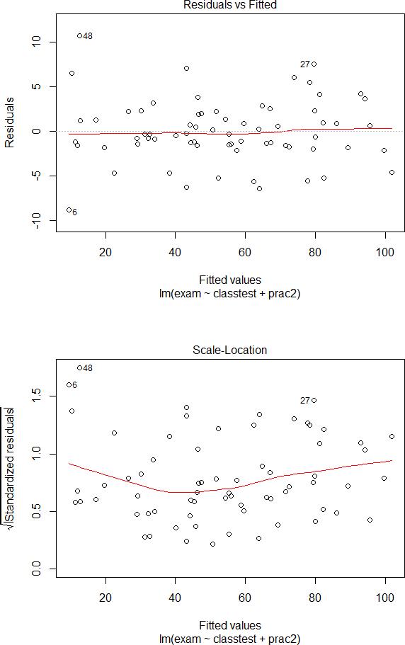
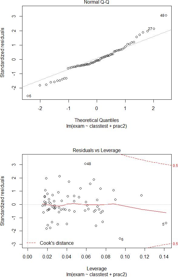
> plot(exammod2)
Residual standard error: 3.608 on 65 degrees of freedom Multiple R-squared: 0.9795,Adjusted R-squared: 0.9789 F-statistic: 1552 on 2 and 65 DF, p-value: < 2.2e-16
> plot(exammod2)
> predict.lm(exammod2, interval=’confidence’)
> predict.lm(exammod2, interval=’confidence’)
fit lwr upr
1 73.950911 72.469522 75.43230
2 69.298596 68.229056 70.36814
3 62.302653 61.276999 63.32831
4 67.131975 65.186678 69.07727
5 22.572596 19.860182 25.28501
6 9.632061 7.417275 11.84685
7 45.468468 44.092766 46.84417
8 43.093585 42.139706 44.04746
9 101.838797 99.845094 103.83250
10 46.412165 45.450833 47.37350
…
66 92.930217 85.533281 100.32715
67 80.085704 72.627145 87.54426
68 43.067245 35.779888 50.35460
(a)Using the R output for the numerical estimates of the regression param- eters,state the fitted models for exammod1 and exammod2. Clearly define any notation you use. [3] 统计推断代考
(b)Explainwhy the lecturer has excluded the first practical mark from model
exammod2, but has retained the other terms. [3]
(c)State the assumptions of fitting the models and running t-tests on the parameters. [2]
(d)Do these assumptions seem reasonablefor exammod2? [4]
(e)Recalling that the exam marks are expressed as a percentage, what short- coming of the model is revealed by the fitted values and corresponding intervals? [2]