
Reports on Stochastic Integral for Continuous-time random walk
概率论代写 The continuous time random walk (CTRW) is defined as a pure jump stochastic process, and the jumps are usually considered instantaneous.
1. Introduction 概率论代写
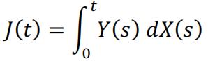
In scientific research and some finance applications, there are need to investigate a stochastic process from an integral angle, and that is to calculate the following equation:
 (1)
(1)
where and are stochastic processes. A traditional Riemann-Stieltjes integral may not be well defined for such a stochastic integral because could be neither continuous nor bounded. being a Brownian motion is a good example of such difficulty. 概率论代写In this report we focus on when and are continuous time random walk processes, and how an integral may defined above may be calculated according to related literatures. To define stochastic integral, we would need to define continuous time random walk, and build on top of this concept, finally we will investigate some examples and numerical methods.
2. Continuous-time random walk
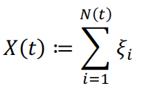
The continuous time random walk (CTRW) is defined as a pure jump stochastic process, and the jumps are usually considered instantaneous. Let denotes a CTRW at time t, X(t) will be the sum of all the jumps occurred before time t:
 (2)
(2)
Where denotes the number of jumps occurred before time t, and denotes the value of jump happened at . CTRW was first introduced in physics by [1], further assumptions are made in the model:
(1)The inter jump time (waiting time) are positive i.i.d. random variables.
(2)The jumps ξi are i.i.d. random variables. They can be extended in vector format to model multi dimension stochastic processes.
(3)ξi and τi can be in different probability families. 概率论代写
So a CTRW can be seemed as a step function: after waiting for a random time, the process will jump up or down a random amount, and it repeats this process. And its current position is the sum of all of the jumps occurred till current time. This definition has a wide application in physics ( modelling particle movements ) and finance alike ( stock price movement ).

3. The Stochastic Integral defined for CTRW
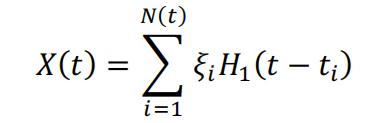
As discussed in the introduction, because a stochastic process could neither continuous nor bounded, the definition of integral in equation (1) is not well defined. The paper by Guido Germano et al. [2] first rewrote equation (2) to with Heaviside’s unit step function in order to define the derivative of X(t), then derived the integral based on it. The details are briefly introduced here:
First equation (2) can be rewritten with Heaviside’s unit step function:
 (3)
(3)
Where Heaviside’s unit step function is defined by:
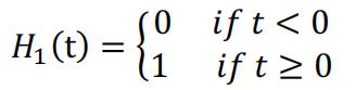
There are also other variants of Heaviside’s unit step function that should return 0 or 1/2 when t = 0. For functions that are right-continuous, this specific one is chosen. So the derivative of X(t) can be defined with Dirac’s function:
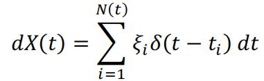 (4)
(4)
In equation (2), the are defined as the values of jumps, here they are rewritten in a right-continuous manner:

Before inserting equation (4) into equation (1), we should also consider the value of . As in Riemann-Stieltjes integral, when dealing with continuous function, we can show that the integral will always have the same value no matter we are evaluating Y(t) at the right / middle or left of the infinitesimal interval . The 3 methods should return the same value of integral when . However, in stochastic process this is not the case because Y(t) is also a stochastic process with jump. Assume we will evaluate Y(t) as , which is a linear interpolation in the infinitesimal interval around t, we can define:
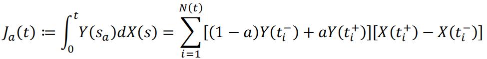
In more general cases, one may choose to evaluate Y(t) as with different value of a. And different Heaviside’s step function may be chosen to define dX(t) as well. The paper [2] introduced the special case to let a = 0, so Y(t) is always adapted, and therefore the integral is a martingale, given CTRW is defined to be right-continuous. And that is:
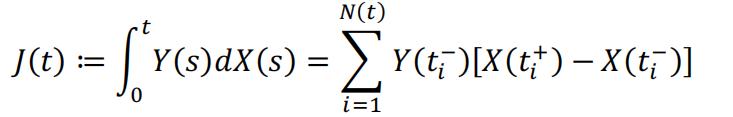 Given equation (6), the integral now is converted into an exact summation.
4. The parameter a and theta’s choice
In defining the integral for stochastic process in section 2, we chose the parameter for the Heaviside’s step function, and we chose a = 1 when evaluating Y(t) in the infinitesimal interval around t. Obviously there are other choices of theta and a’s, here we will summarize their relative applications:
1.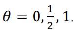
Usually we will choose for right continuous function and for left continuous function so we can have well defined at the random jumps. Some may choose 1/2 for symmetry of the function. But after we arrive at equation (6), the choice mostly doesn’t matter as the jumps happen for countable times, and the measure of these point set is zero.
2. a ∈ [0,1]
When a = 0, we evaluate Y(t) at the “left point” of the infinitesimal interval around t, the integral is called Ito integral. And when a = 1, we evaluate Y(t) at the “right point” of that. We will also call the integral when a=1/2 the Stratonovich integral. Different from a Riemann integral, the choice of a can have a big different for stochastic integral. See the example below:
Example 1
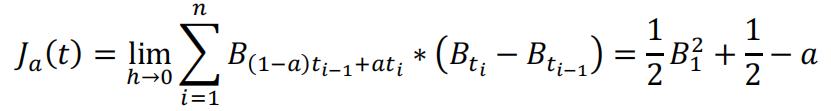
To calculate ∫01 Bt dBt, where Bt is a standard Brownian motion, a continuous time random walk. Following equation (5), we have that:
Where t = nh. t1 = i ∗ ℎ, i = 0,1,2,3 … n.It’s clear that for different choices of a, the result will be different. An intuitive explanation would be that when a = 1, we evaluate on the right point. And that ‘enables looking into the future’. Most financial application of stochastic process choose a=0 because the Ito integral has a martingale property. Further detail are discussed in von Jouanne-Diedrich[3].
5. Numerical Application 概率论代写
The definition of this stochastic integral of CTRW based on exact summations encourages us to apply such technique in numerical methods. In some applications such as finance, Monte Carlo simulation are frequently used to evaluate a stochastic integral. For example, let’s assume X(t) is a stochastic process with a stochastic differential equation:
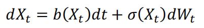
Where is a Wiener process. The solution to this SDE is a stochastic integral:
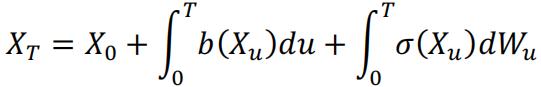
The last part of the integral can be evaluate using equation (6). However, to obtain a numerical solution on or more complex function , Monte Carlo simulation is an effective method.
Simulation usually involves discretization, and that is to split the interval into small intervals. And when the interval is small enough, we can approximate equation (4). For the example we gave above, the discretization is be:

And the Euler scheme to generate the random path for X is:
- Let h be a sufficiently small number, n = t/h.
- Generate n independent N(0,1) random variables
- Compute iteratively:
![]()
It’s trivial to see that this is a direct application of equation (6) in section 3.
And for a more accurate Milstein scheme, we can use this formula for the iteration:

The quadratic term is from Taylor’s expansion of the original SDE. This makes Milstein scheme converges faster than Euler’s scheme.
However, in practical calculation, these two schemes hardly make a difference, and Milstein scheme may have issue when simulating multi-dimensional stochastic process. One of the difficult examples is to calculate:
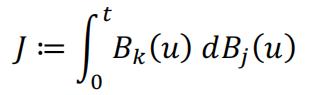
Where are different components of a multi-dimensional Brownian motion. There is no straightforward way to generate the quadratic term.
6. Conclusion 概率论代写
In this report we reviewed the definition and detail of stochastic integral on continuous time random walk and its application. Future work will be studying the convergence speed and methods to reduce variance when evaluating a stochastic integral using Monte Carlo methods.
______________________________
[1] E. Montroll and G. H. Weiss, J. Math. Phys. 6, 167 (1965). [2] Germano, G., Politi, M., Scalas, E., & Schilling, R.L. (2009). Stochastic calculus for uncoupled continuous-time random walks. Physical review. E, Statistical, nonlinear, and soft matter physics, 79 6 Pt 2, 066102 . [3] von Jouanne-Diedrich, Holger, Ito, Stratonovich and Friends (May 18, 2017). Available at SSRN: https://ssrn.com/abstract=2956257 or http://dx.doi.org/10.2139/ssrn.2956257
更多代写:留学生计算机作业代写 多邻国代考 留学生代写assignment 留学生代写 留学生代写论文 代写MBA论文价格
