STAT 321 – Regression and Forecasting (non-specialist)
Final Assessment – W21
回归和预测代做 Total Marks Available: 65 Clarifying questions are not permitted. Please read each question carefully. Show your work.
Total Marks Available: 65
- Clarifying questions are not permitted.
- Please read each question carefully. Show your work. Your grade will be influenced by how clearly you express your ideas, and how well you organize your solutions.
1)
The output below is from four linear regression models fit to data (n = 102) on stock liquidity, as measured by trading VOLUME (millions of shares), and other financial characteristics, including:
PRICE: Opening stock price ($)
NTRAN: Three months total number of transactions
SHARE: Number of outstanding shares (millions of shares)
VALUE Market equity value (millions of dollars)
DEBEQ: Debt-to-equity ratio
Note that to address issues with model adequacy, a square root transformation was used on the response and on all the explanatory variables.
Model 1:(sqrt(VOLUME)~sqrt(NTRAN)+sqrt(PRICE)+sqrt(SHARE)+sqrt(VALUE)+sqrt(DEBEQ)) 回归和预测代做
             Estimate Std. Error t value Pr(>|t|)
(Intercept) -0.139640 0.376454 -0.371 0.7115
sqrt(NTRAN)  0.038132 ******** 12.661 <2e-16
sqrt(PRICE)  0.011692 ********  0.218 0.8283
sqrt(SHARE)  0.082470 ********  2.125 0.0361
sqrt(VALUE) -0.117631 ******** -0.704 0.4830
sqrt(DEBEQ)  0.057191 ********  1.155 0.2508
Multiple R-squared: 0.8753, Adjusted R-squared: *****
Model 2 (sqrt(VOLUME)~sqrt(NTRAN)+sqrt(PRICE)+sqrt(VALUE)+sqrt(DEBEQ))
             Estimate Std. Error t value Pr(>|t|)
(Intercept)  0.380432 ********  1.306 0.1945
sqrt(NTRAN)  0.039924 ******** 13.565 <2e-16
sqrt(PRICE) -0.068192 ******** -1.743 0.0845
sqrt(VALUE)  0.193577 ********  2.367 0.0199
sqrt(DEBEQ)  0.065178 ********  1.297 0.1976
Residual standard error: 0.5109 on 97 degrees of freedom
Multiple R-squared: 0.8695, Adjusted R-squared: *****
Model 3 (sqrt(VOLUME) ~ sqrt(NTRAN) + sqrt(PRICE) + sqrt(VALUE))
             Estimate Std. Error t value Pr(>|t|)
(Intercept)  0.479634 0.281969  1.701 0.0921
sqrt(NTRAN)  0.039861 ******** 13.499 <2e-16
sqrt(PRICE) -0.068314 ******** -1.740 0.0850
sqrt(VALUE)  0.188293 ********  2.297 0.0237
Residual standard error: *******
Multiple R-squared: 0.8672, Adjusted R-squared: 0.8631
Model 4 (sqrt(VOLUME) ~ sqrt(PRICE))
            Estimate Std. Error t value Pr(>|t|)
(Intercept) 2.62506 0.51607 5.087 1.71e-06
sqrt(PRICE) 0.12147 0.08331 1.458    0.148
Residual standard error: 1.378
F-statistic: ***** on ** and ** DF, p-value: *****
a) 回归和预测代做
Graphical evidence suggested that multicollinearity may be an issue, particularly with the sqrt(SHARE) variable. Further analysis yielded a VIF for this variable of 12.59.
i) [3] What proportion of the variation in sqrt(SHARE) is accounted for by the other explanatory variables?
ii) [2] What is the ‘graphical evidence’ referred to in the question? Explain.
iii) [1] What do you conclude from the VIF?
iv) [2] What effect do you expect the removal of the SHARE variable will have on the remaining parameter estimators?
b) 回归和预测代做
Consider the following partial anova output from a comparison of Model 4 to Model 2:
 > anova(Model 4, Model 2)
Analysis of Variance Table
Model 1: sqrt(VOLUME)~sqrt(PRICE)
Model 2: sqrt(VOLUME)~sqrt(NTRAN)+sqrt(PRICE)+sqrt(VALUE)+sqrt(DEBEQ)
  Res.Df     RSS   Df   Sum of Sq      F     Pr(>F)

1 ____ __________

2 ____ ___________ ____ ___________ _____  < 2.2e-16
i) [5] Fill in the table by finding the missing values (those displayed with a ‘______’ ). Show your work!
ii) [1] State the null hypothesis for this test.
iii) [2] Clearly state the conclusion of this test in the context of the study
c) [2]
Consider Model 3. Put the margin of error associated with a confidence interval for the parametersb1,b2, b3 in increasing order. Justify your answer.
d) [2]
Consider Model 4. A 95% prediction interval for the (sqrt) volume of a stock with a certain price is given by:
   fit       lwr      upr
****** 0.6812053 6.180445
Give the price (in $) of this stock. Show your work.
e) [2]
Give the F statistic and associated p-value for Model 4. Minimal calculations are required.
ii) [3] Mallows’ Cp (Note that Model 2 is the ‘full’ model here)
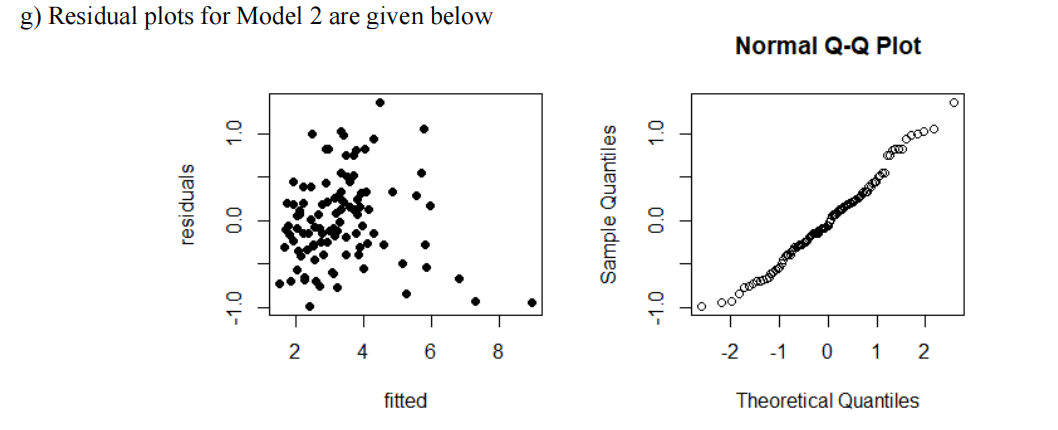
i) [3] Comment on the adequacy of the model, as it relates to model assumptions.
ii) [3] The stock with the largest estimated mean volume in the above plot is associated with a leverage = 0.366. Is this an influential observation? Show your work (the value of the relevant residual can be estimated from the plot).
2) 回归和预测代做
Consider the regression model fit to data from the Waterloo faculty salary study in which researchers wished to determine whether there was a systemic discrepancy in salary between male and female faculty members. Partial regression output is shown below (the response variable was annual salary ($)).
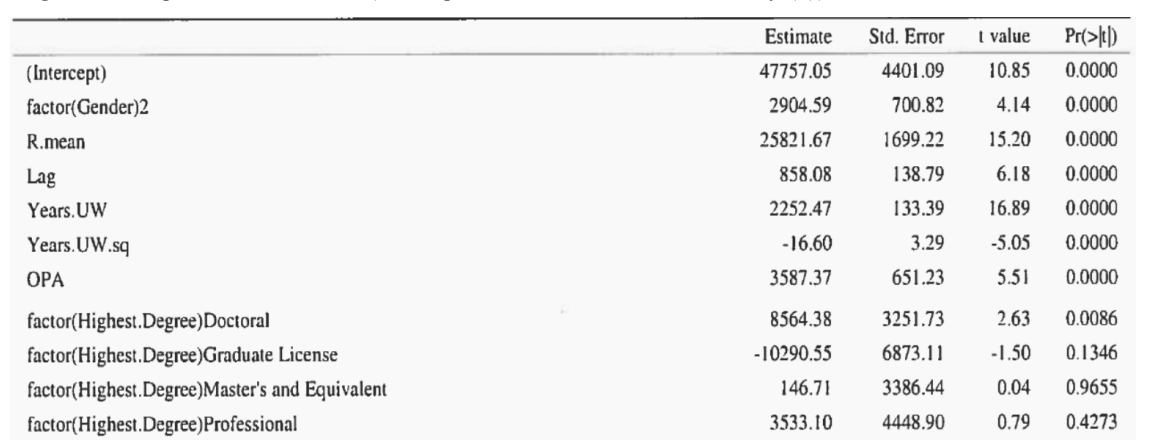
a) [2] By how much did they raise the salary of female faculty members? Briefly explain their rationale.
b) Note that the Highest Degree variable consists of the five levels: Doctoral, Graduate License, Master’s and Equivalent, Professional, and Bachelor.
i) [3] Interpret the Doctoral parameter estimate in the context of the study.
ii) [3] From the p-values, briefly summarize what has been learned about the relationships between highest degree obtained and salary.
3) 回归和预测代做
Below is output from a regression model fit to a time series on quarterly sales (in millions of dollars) for the Disney company over a 14 year period (from the first quarter of 1981 to the last quarter of 1994). Note that log(Sales) was used as the response:
Call: lm(formula = log(Sales) ~ dis.quart + t)
Coefficients:
               Estimate Std. Error t value Pr(>|t|)
(Intercept)   5.3651647 0.0398077 134.777 <2e-16
dis.quartQ1  -0.0210920 0.0413082  -0.511 0.612
dis.quartQ2   0.0351646 0.0412587   0.852 0.398
dis.quartQ3   0.0594174 0.0412290   1.441 0.156
t             0.0472373 0.0009038  52.266 <2e-16
Residual standard error: 0.1091 on 51 degrees of freedom
Multiple R-squared: 0.9818, Adjusted R-squared: 0.9804
a) [3] ForecastY57the sales (in dollars) for the first quarter of 1995.
b) Suppose you wish to perform an additional sum of squares test to investigate whether there is a difference in mean sales between Quarter 2 and Quarter 3, after accounting for trend.
i) [3] Provide the full and reduced models for this test. Be sure to define all explanatory variables in both models.
ii) [2] Give the null hypothesis in the formH0: Aβ = 0
iii) [2] Based on the above output and by consulting the appropriate probability table, make an educated guess as to the approximate value of the test statistic. No calculations are required.
c) [3] It was found that the assumption of independence of the errors was not valid. Briefly describe two methods that could lead to this conclusion.
d) An AR(1) model was fit to the residuals, yielding the output below:
Call: arima(x = residuals(dis.lm), order=c(1,0,0), include.mean=FALSE)
Coefficients:
         ar1
      0.2957
s.e.  0.1276
sigma^2 estimated as 0.009871:
Sales for the last quarter of 1994 was $3.3017 × 10⁹ (just over 3.3 billion dollars)
i) [5] Forecaste57(you do not have to give the units).
ii) [2] Use the forecasted value ofe57to revise your forecast of Y57 in a). Report your forecast in dollars.
4) 回归和预测代做
[2] One method to account for the seasonal and trend component in a time series is with a linear regression model. Another method is differencing. Describe, with reference to the backshift operator, how differencing might be employed in the Disney sales series to eliminate both the seasonal and trend components.
5)
[2] We have seen that smoothing methods are often used in graphical displays of the daily number of new Covid-19 cases in a particular region. At the time of this exam, new cases continue to rise in Ontario. In the presence of such a trend, which of the two smoothing methods (moving average, EWMA) would likely lead to a lower MSE, and why?