
Project 5 – Machine Learning – CS 188: Introduction to Artificial Intelligence, Spring 2021
代写Machine Learning作业 Submit machinelearning.token , generated by running submission_autograder.py , to Project 5 on Gradescope.
Project 5: Machine Learning
In this project you will build a neural network to classify digits, and more!
Introduction 代写Machine Learning作业
This project will be an introduction to machine learning.
The code for this project contains the following fifiles, available as a zip archive.
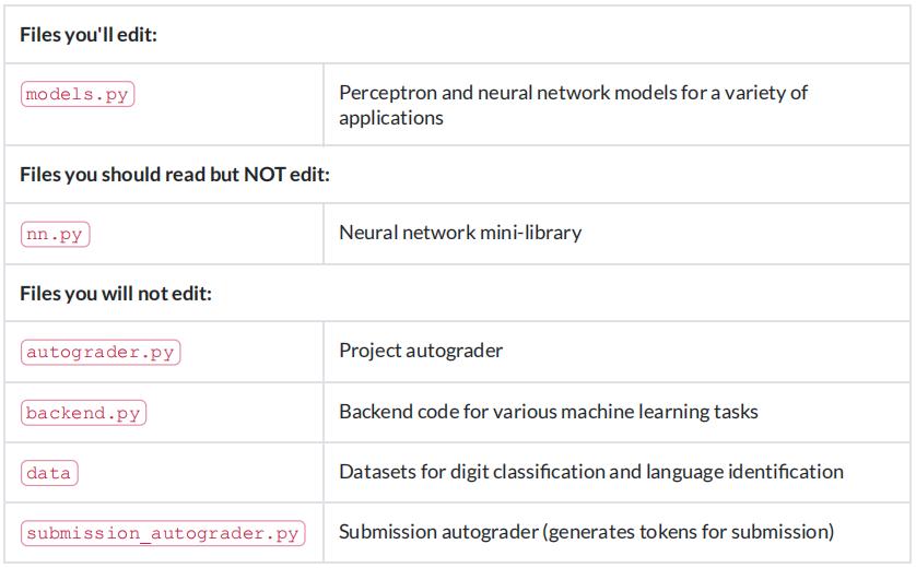
Files to Edit and Submit: You will fifill in portions of models.py during the assignment. Please do not change the other fifiles in this distribution.
Note: You only need to submit machinelearning.token , generated by running submission_autograder.py . It contains the evaluation results from your local autograder, and a copy of all your code. You do not need to submit any other fifiles. See Submission for details.
Evaluation: Your code will be autograded for technical correctness. Please do not change the names of any provided functions or classes within the code, or you will wreak havoc on the autograder. However,the correctness of your implementation – not the autograder’s judgements – will be the fifinal judge of your score. If necessary, we will review and grade assignments individually to ensure that you receive due credit for your work. 代写Machine Learning作业
Academic Dishonesty: We will be checking your code against other submissions in the class for logical redundancy.
If you copy someone else’s code and submit it with minor changes, we will know. These cheat detectors are quite hard to fool, so please don’t try. We trust you all to submit your own work only; please don’t let us down. If you do, we will pursue the strongest consequences available to us.
Proper Dataset Use: Part of your score for this project will depend on how well the models you train perform on the test set included with the autograder. We do not provide any APIs for you to access the test set directly. Any attempts to bypass this separation or to use the testing data during training will be considered cheating.
Getting Help: You are not alone! If you fifind yourself stuck on something, contact the course staff for help.Offifice hours, section, and the discussion forum are there for your support; please use them. If you can’t make our offifice hours, let us know and we will schedule more. We want these projects to be rewarding and instructional, not frustrating and demoralizing. But, we don’t know when or how to help unless you ask.
Discussion: Please be careful not to post spoilers.
Installation
For this project, you will need to install the following two libraries:
numpy, which provides support for large multi-dimensional arrays – installation instructions matplotlib, a 2D plotting library – installation instructions
If you have a conda environment, you can install both packages on the command line by running:
conda activate [your environment name]
pip install numpy
pip install matplotlib
You will not be using these libraries directly, but they are required in order to run the provided code and autograder.
To test that everything has been installed, run:
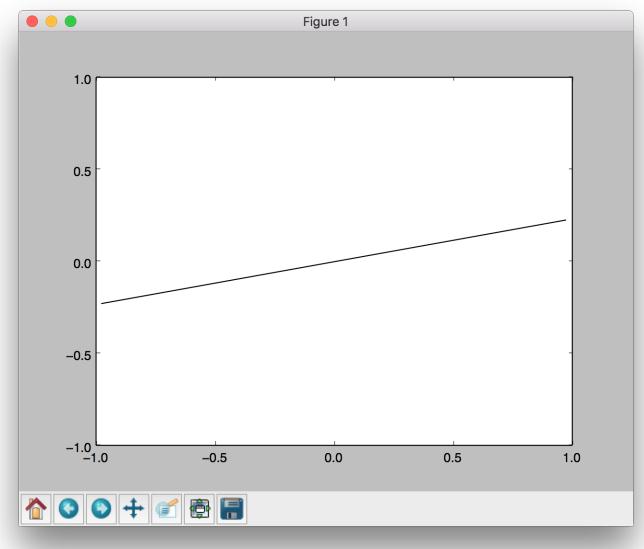
python autograder.py --check-dependencies
If numpy and matplotlib are installed correctly, you should see a window pop up where a line segment spins in a circle:
Provided Code (PartI)
For this project, you have been provided with a neural network mini-library ( nn.py ) and a collection of datasets ( backend.py ).
The library in nn.py defifines a collection of node objects. Each node represents a real number or a matrix of real numbers. Operations on node objects are optimized to work faster than using Python’s built-in types (such as lists).
Here are a few of the provided node types:
- nn.Constant represents a matrix (2D array) of flfloating point numbers. It is typically used to represent input features or target outputs/labels. Instances of this type will be provided to you by other functions in the API; you will not need to construct them directly.
- nn.Parameter represents a trainable parameter of a perceptron or neural network.
- nn.DotProduct computes a dot product between its inputs.
- Additional provided functions:
- nn.as_scalar can extract a Python flfloating-point number from a node.
When training a perceptron or neural network, you will be passed a dataset object. You can retrieve batches of training examples by calling dataset.iterate_once(batch_size) :
for x, y in dataset.iterate_once(batch_size):

...
For example, let’s extract a batch of size 1 (i.e., a single training example) from the perceptron training data:
>>> batch_size = 1

>>> for x, y in dataset.iterate_once(batch_size):

... print(x)

... print(y)

... break

...

<Constant shape=1x3 at 0x11a8856a0>

<Constant shape=1x1 at 0x11a89efd0>
The input features x and the correct label y are provided in the form of nn.Constant nodes. The shape of x will be batch_size x num_features , and the shape of y is batch_size x num_outputs . Here is an example of computing a dot product of x with itself, fifirst as a node and then as a Python number. 代写Machine Learning作业
Question 1 (8 points): Perceptron
Before starting this part, be sure you have numpy and matplotlib installed!
In this part, you will implement a binary perceptron. Your task will be to complete the implementation of the PerceptronModel class in models.py .
For the perceptron, the output labels will be either or , meaning that data points (x, y) from the dataset will have y be a nn.Constant node that contains either or as its entries. You can check last semester’s note 9 pages 10-13 for an example of a +1/-1 perceptron.
We have already initialized the perceptron weights self.w to be a parameter node.
The provided code will include a bias feature inside x when needed, so you will not need a separate parameter for the bias.
Your tasks are to:
- Implement the run(self, x) method. This should compute the dot product of the stored weight vector and the given input, returning an nn.DotProduct object.
- Implement get_prediction(self, x) , which should return if the dot product is non-negative or otherwise. You should use nn.as_scalar to convert a scalar Node into a Python flfloating-point number.
- Write the train(self) method. This should repeatedly loop over the data set and make updates on examples that are misclassifified. Use the update method of the nn.Parameter class to update the weights. When an entire pass over the data set is completed without making any mistakes, 100% training accuracy has been achieved, and training can terminate.
In this project, the only way to change the value of a parameter is by calling parameter.update(direction, multiplier) , which will perform the update to the weights:
weights ← weights + direction ⋅ multiplier
The direction argument is a Node with the same shape as the parameter, and the multiplier argument is a Python scalar.
To test your implementation, run the autograder:
python autograder.py -q q1
Note: the autograder should take at most 20 seconds or so to run for a correct implementation. If the autograder is taking forever to run, your code probably has a bug.

Neural Network Tips
In the remaining parts of the project, you will implement the following models:
Q2: Regression
Q3: Handwritten Digit Classifification
Q4: Language Identifification
Building Neural Nets 代写Machine Learning作业
Throughout the applications portion of the project, you’ll use the framework provided in nn.py to create neural networks to solve a variety of machine learning problems. A simple neural network has layers, where each layer performs a linear operation (just like perceptron). Layers are separated by a non-linearity, which allows the network to approximate general functions. We’ll use the ReLU operation for our non-linearity, defifined as . For example, a simple two-layer neural network for mapping an input row vector to an output vector would be given by the function:
![]()
where we have parameter matrices and and parameter vectors and to learn during gradient descent. will be an matrix, where is the dimension of our input vectors , and is the hidden layersize. will be a size vector. We are free to choose any value we want for the hidden size(we will just need to make sure the dimensions of the other matrices and vectors agree so that we can perform the operations). Using a larger hidden size will usually make the network more powerful (able to fifit more training data), but can make the network harder to train (since it adds more parameters to all the matrices and vectors we need to learn), or can lead to overfifitting on the training data.We can also create deeper networks by adding more layers, for example a three-layer net:
![]()
Note on Batching
For effificiency, you will be required to process whole batches of data at once rather than a single example at a time. This means that instead of a single input row vector with size , you will be presented with a batch of inputs represented as a matrix . We provide an example for linear regression to demonstrate how a linear layer can be implemented in the batched setting.
Note on Randomness 代写Machine Learning作业
The parameters of your neural network will be randomly initialized, and data in some tasks will be presented in shufflfled order. Due to this randomness, it’s possible that you will still occasionally fail some tasks even with a strong architecture – this is the problem of local optima! This should happen very rarely, though – if when testing your code you fail the autograder twice in a row for a question, you should explore other architectures.
Practicaltips
Designing neural nets can take some trial and error. Here are some tips to help you along the way:
- Be systematic. Keep a log of every architecture you’ve tried, what the hyperparameters (layer sizes,learning rate, etc.) were, and what the resulting performance was. As you try more things, you can start seeing patterns about which parameters matter. If you fifind a bug in your code, be sure to cross out past results that are invalid due to the bug.
- Start with a shallow network (just two layers, i.e. one non-linearity). Deeper networks have exponentially more hyperparameter combinations, and getting even a single one wrong can ruin your performance. Use the small network to fifind a good learning rate and layer size; afterwards you can consider adding more layers of similar size.
- If your learning rate is wrong, none of your other hyperparameter choices matter. You can take a state-of-the-art model from a research paper, and change the learning rate such that it performs no better than random. A learning rate too low will result in the model learning too slowly, and a learning rate too high may cause loss to diverge to infifinity. Begin by trying different learning rates while looking at how the loss decreases over time. 代写Machine Learning作业
-
Smaller batches require lower learning rates. When experimenting with different batch sizes, be aware that the best learning rate may be different depending on the batch size.
- Refrain from making the network too wide (hidden layer sizes too large) If you keep making the network wider accuracy will gradually decline, and computation time will increase quadratically in the layer size – you’re likely to give up due to excessive slowness long before the accuracy falls too much. The full autograder for all parts of the project takes 2-12 minutes to run with staff solutions;if your code is taking much longer you should check it for effificiency.
- If your model is returning Infifinity or NaN, your learning rate is probably too high for your current architecture.
- Recommended values for your hyperparameters:
Hidden layer sizes: between 10 and 400.
Batch size: between 1 and the size of the dataset. For Q2 and Q3, we require that total size of the dataset be evenly divisible by the batch size.
Learning rate: between 0.001 and 1.0.
Number of hidden layers: between 1 and 3.
Provided Code (PartII) 代写Machine Learning作业
Here is a full list of nodes available in nn.py . You will make use of these in the remaining parts of the assignment:
- nn.Constant represents a matrix (2D array) of flfloating point numbers. It is typically used to represent input features or target outputs/labels. Instances of this type will be provided to you by other functions in the API; you will not need to construct them directly.
- nn.Parameter represents a trainable parameter of a perceptron or neural network. All parameters must be 2-dimensional.
Usage: nn.Parameter(n, m) constructs a parameter with shape n × m
- nn.Add adds matrices element-wise.
Usage: nn.Add(x, y) accepts two nodes of shape batch_size × num_features and constructs a node that also has shape batch_size × num_features.
- nn.AddBias adds a bias vector to each feature vector.
Usage: nn.AddBias(features, bias) accepts features of shape batch_size × num_features and bias of shape , and constructs a node that has shape batch_size × num_features.
- nn.Linear applies a linear transformation (matrix multiplication) to the input.
Usage: nn.Linear(features, weights) accepts features of shape and weights of shape, and constructs a node that has shape.
- nn.ReLU applies the element-wise Rectifified Linear Unit nonlinearity relu(x) = max(x, 0).This nonlinearity replaces all negative entries in its input with zeros.
Usage: nn.ReLU(features) , which returns a node with the same shape as the input .
-
nn.SquareLoss computes a batched square loss, used for regression problems
Usage: nn.SquareLoss(a, b) , where a and b both have shape batch_size × num_outputs.
- nn.SoftmaxLoss computes a batched softmax loss, used for classifification problems.
Usage: nn.SoftmaxLoss(logits, labels) , where logits and labels both have shape batch_size × num_classes. The term “logits” refers to scores produced by a model, where each entry can be an arbitrary real number. The labels, however, must be non-negative and have each row sum to 1. Be sure not to swap the order of the arguments! 代写Machine Learning作业
- Do not use nn.DotProduct for any model other than the perceptron.
The following methods are available in nn.py :
- nn.gradients computes gradients of a loss with respect to provided parameters.
Usage:
nn.gradients(loss, [parameter_1, parameter_2, …, parameter_n]) will return a list [gradient_1, gradient_2, …, gradient_n] , where each element is an nn.Constant containing the gradient of the loss with respect to a parameter.
- nn.as_scalar can extract a Python flfloating-point number from a loss node. This can be useful to determine when to stop training.
Usage: nn.as_scalar(node) , where node is either a loss node or has shape (1,1) .The datasets provided also have two additional methods:
- dataset.iterate_forever(batch_size) yields an infifinite sequences of batches of examples.
- dataset.get_validation_accuracy() returns the accuracy of your model on the validation set. This can be useful to determine when to stop training.
Example: Linear Regression
As an example of how the neural network framework works, let’s fifit a line to a set of data points. We’ll start four points of training data constructed using the function . In batched form, our data is:
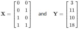
and
Suppose the data is provided to us in the form of nn.Constant nodes:
>>> x

<Constant shape=4x2 at 0x10a30fe80>

>>> y

<Constant shape=4x1 at 0x10a30fef0>
Let’s construct and train a model of the form f(x) = x0 ⋅ m0 + x1 ⋅ m1 + b. If done correctly, we should be able to learn than m0 = 7, m1 = 8, and b = 3. 代写Machine Learning作业
First, we create our trainable parameters. In matrix form, these are:
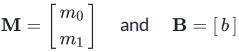
Which corresponds to the following code:
m = nn.Parameter(2, 1)

b = nn.Parameter(1, 1)
Printing them gives:
>>> m

<Parameter shape=2x1 at 0x112b8b208>

>>> b

<Parameter shape=1x1 at 0x112b8beb8>
Next, we compute our model’s predictions for y:
xm = nn.Linear(x, m)

predicted_y = nn.AddBias(xm, b)
Our goal is to have the predicted y-values match the provided data. In linear regression we do this by minimizing the square loss:![]()
We construct a loss node:
loss = nn.SquareLoss(predicted_y, y)
In our framework, we provide a method that will return the gradients of the loss with respect to the parameters:
grad_wrt_m, grad_wrt_b = nn.gradients(loss, [m, b])
Printing the nodes used gives:
>>> xm

<Linear shape=4x1 at 0x11a869588>

>>> predicted_y

<AddBias shape=4x1 at 0x11c23aa90>

>>> loss

<SquareLoss shape=() at 0x11c23a240>

>>> grad_wrt_m

<Constant shape=2x1 at 0x11a8cb160>

>>> grad_wrt_b

<Constant shape=1x1 at 0x11a8cb588>
We can then use the update method to update our parameters. Here is an update for m , assuming we have already initialized a multiplier variable based on a suitable learning rate of our choosing:
m.update(grad_wrt_m, multiplier)
If we also include an update for b and add a loop to repeatedly perform gradient updates, we will have the full training procedure for linear regression.
Question 2 (8 points): Non-linear Regression
For this question, you will train a neural network to approximate sin(x) [−2π, 2π].
You will need to complete the implementation of the RegressionModel class in models.py . For this problem, a relatively simple architecture should suffifice (see Neural Network Tips for architecture tips.)Use nn.SquareLoss as your loss.
While we are fifinalizing neural network notes for this semester, you can take a look at the previous semester’s neural network notes. 代写Machine Learning作业
Your tasks are to:
- Implement RegressionModel.__init__ with any needed initialization
- Implement RegressionModel.run to return a node that represents your model’s prediction.
- Implement RegressionModel.get_loss to return a loss for given inputs and target outputs.
- Implement RegressionModel.train , which should train your model using gradient-based updates.
There is only a single dataset split for this task (i.e., there is only training data and no validation data or test set). Your implementation will receive full points if it gets a loss of 0.02 or better, averaged across all examples in the dataset. You may use the training loss to determine when to stop training (use nn.as_scalar to convert a loss node to a Python number). Note that it should take the model a few minutes to train.
Question 3 (9 points): Digit Classifification
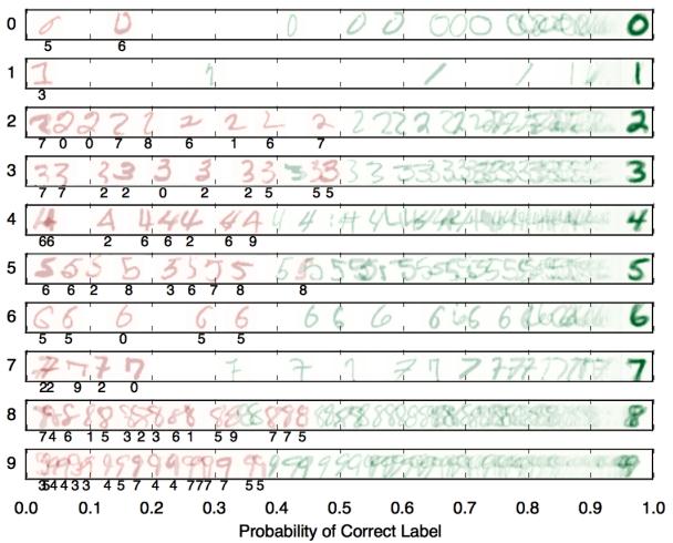
For this question, you will train a network to classify handwritten digits from the MNIST dataset.
Each digit is of size pixels, the values of which are stored in a -dimensional vector of flfloating point numbers. Each output we provide is a 10-dimensional vector which has zeros in all positions, except for a one in the position corresponding to the correct class of the digit. 代写Machine Learning作业
Complete the implementation of the DigitClassificationModel class in models.py . The return value from DigitClassificationModel.run() should be a node containing scores,where higher scores indicate a higher probability of a digit belonging to a particular class (0-9). You should use nn.SoftmaxLoss as your loss. Do not put a ReLU activation after the last layer of the network.
For both this question and Q4, in addition to training data, there is also validation data and a test set.
You can use dataset.get_validation_accuracy() to compute validation accuracy for your model,which can be useful when deciding whether to stop training. The test set will be used by the autograder.
To receive points for this question, your model should achieve an accuracy of at least 97% on the test set.For reference, our staff implementation consistently achieves an accuracy of 98% on the validation data after training for around 5 epochs. Note that the test grades you on test accuracy, while you only have access to validation accuracy – so if your validation accuracy meets the 97% threshold, you may still fail the test if your test accuracy does not meet the threshold. Therefore, it may help to set a slightly higher stopping threshold on validation accuracy, such as 97.5% or 98%.
To test your implementation, run the autograder:
python autograder.py -q q3
Submission 代写Machine Learning作业
Submit machinelearning.token , generated by running submission_autograder.py , to Project 5 on Gradescope.
The full project autograder takes 2-12 minutes to run for the staff reference solutions to the project. If your code takes signifificantly longer, consider checking your implementations for effificiency.
Note: You only need to submit machinelearning.token , generated by running submission_autograder.py . It contains the evaluation results from your local autograder, and a copy of all your code. You do not need to submit any other fifiles.
Please specify any partner you may have worked with and verify that both you and your partner are associated with the submission after submitting.

更多代写:Online Test代考多少钱 report写作 Quiz/Exam代考 留学essay代写美国 Position Paper代写 计算机网课作业代写
