
COMS 4771 HW2 (Spring 2022)
代写机器学习 Let M−denote the total number of mistakes on negative examples, and T W (t) denote the total weight of w at iteration t.
This homework is to be done alone. No late homeworks are allowed. To receive credit, a type- setted copy of the homework pdf must be uploaded to Gradescope by the due date. You must show your work to receive full credit. Discussing possible approaches for solutions for homework ques- tions is encouraged on the course discussion board and with your peers, but you must write their own individual solutions and not share your written work/code. You must cite all resources (includ- ing online material, books, articles, help taken from/given to specific individuals, etc.) you used to complete your work.
1 A variant of Perceptron Algorithm
One is often interested in learning a disjunction model. That is, given binary observations from a d feature space (i.e. each datapoint x ∈ {0, 1} d), the output is an ‘OR’ of few of these features (e.g. y = x1 ∨ x20 ∨ x33). It turns out that the following variant of the perceptron algorithm can learn such disjunctions well.
Perceptron OR Variant
learning:
-Initialize w :=1
-foreach datapoint (x, y) in the training dataset
– yˆ := 1[w · x > d]
-ify ≠ yˆ and y = 1
-wi← 2wi (for ∀i : xi = 1)
-ify≠ yˆ and y = 0 代写机器学习
-wi← wi/2 (for ∀i : xi = 1)
classification:
f (x) := 1[w · x > d]
We will prove the following interesting result: The Perceptron OR Variant algorithm makes at -most 2 + 3r(1 + log d) mistakes when the target concept is an OR of r variables.
(i)Show that for any positive example, Perceptron OR Variantmakes M+ r(1 + log d) mistakes.
(ii)Showthat each mistake made on a negative example decreases the total weight  by at least d/2.
(iii)Let M−denote the total number of mistakes on negative examples, and T W (t) denote the total weight of w at iteration t. Observing that
0 < T W (t) ≤ T W (0) + dM+ − (d/2)M−,
conclude that the total number of mistakes (i.e., M+ + M−) is at most 2 + 3r(1 + log d).

2 Understanding the RBF Kernel 代写机器学习
Reca.ll the RBF kernel with parameter γ > 0 which, given x, x′ ∈ Rd, is defined as K(x, x′) =exp ![]() In this question we will try to understand what feature transformation this ker-nel function corresponds to and what makes this kernel function so powerful and useful in practice.
In this question we will try to understand what feature transformation this ker-nel function corresponds to and what makes this kernel function so powerful and useful in practice.
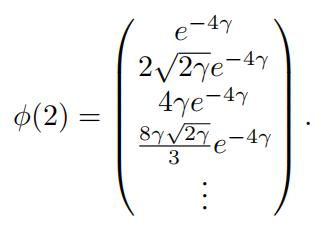
For the sake of simplicity1, assume that d = 1. Let ϕ be the feature transform which maps an input x ∈ R.to an infinite dimensional vector whose ith (i takes on values 0, 1, 2, . . . ) coordinate is 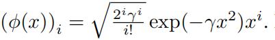 For example ϕ(2) is an infinite dimensional vector whose first few entries are as follows:
We can then define ϕ(x) · ϕ(x′) = Σ∞i=0 ϕ(x)iϕ(x′)i.
(a)Showthat K(x, x′) = ϕ(x) ϕ(x′) for the specific K and ϕ defined above.
Hint: You can use the fact that for any x ∈ R : exp(x) = ![]() (this is just the Taylor series of exp(x)).
(this is just the Taylor series of exp(x)).
Consider any polynomial function g : Rd →R (where again we assume d = 1 for simplicity).
Without loss of generality (which is often abbreviated WLOG and just means that this assumption is always true and so isn’t really an assumption) we can write g(x) = Σm aixpi for some m > 0,coefficients a1, a2 . . . , am ∈ R, and some distinct non-negative integers p1, p2, . . . , pm. 代写机器学习
(b)Show that there is an infinite length vector w such that g(x) = exp γx2w ϕ(x). Con- clude that any polynomial boundary g(x) =0 becomes linear when using the RBF Specifically, show that g(x) = 0 iff w · ϕ(x) = 0 for the w you found.
(c) Look at how the parameter γ affects the coefficients of your vector w from part (b). Use this observation to explain the relationship between γ and over/under-fitting. If you have lots of data and know that the “best” boundary is a high degree polynomial, should γ be big or small?What if you have very little data and are afraid of fitting to noise, should γ be large or small?
1There is a d dimensional equivalent to everything you will show below, and the conclusions are the same. The only difference is that the algebra gets uglier. If that doesn’t scare you, feel free to do this question without the d = 1 assumption (you’ll need to come up with the correct ϕ for d-dimensions and change how we write g).
3 Analyzing Games via Optimization 代写机器学习
Recall the game of rock-paper-scissors. In this game there are two players, p1 and p2, that each choose an element of r, p, s as their only move for the game. One can study such games more systematically. For example, this game can be analyzed by examining the possible moves each player can make and representing the outcomes as a payoff matrix P . In particular, given that p1 plays move i r, p, s and p2 plays move j r, p, s , the resulting game payoff (from the perspective of p1) is the amount Pij. 代写机器学习
(i)What is the payoff matrix for p1in the game of rock paper scissors, where winning results in a payoff of 1, losing a payoff of −1, and a tie a payoff of 0?
(ii)If the matrix Q is the payoff from the perspective of player p2, then what is the relationship between P andQ?
Now consider a game with payoff matrix A 1, 1 n×n (notice, +1 means win, 1 means lose,and there are no ties in this game).
There are two players, p1 and p2, that must choose moves i and j 1, . . . , n , respectively. Similar to rock-paper-scissors, neither p1 nor p2 knows the other’s choice before making their own choice, but they do have access to the payoff A. Following theirchoices of i and j, p1 receives reward Ai,j. Of course, p1’s objective is to receive maximum possiblepayoff, and since p2 and p1 are in competition, p2’s objective is for p1 to receive minimum possible payoff.
(iii)Describe the set of matrices S ⊂ {−1, 1}n×n t. ∀A ∈ S, there exists some choice of i ∈ {1, . . . , n} that guarantees a win for p1 (no more than two sentences are needed). 代写机器学习
If neither p1 nor p2 has a move that can result in a guaranteed win for them, they might have some tough choices to make about how to select their move. Suppose they can each formulate a probabilistic strategy – instead of committing to a particular move as their strategy, they can each define a probability distribution over the moves 1, . . . , n for p1 and p2, as their strategy (meaning, at play time, a move is randomly selected according to the described probability distribution). We can define the strategy of player i as si ∈ Rn, such that si is the probability that player i chooses to play move k. Naturally, we have that ![]()
(iv)Wewill now analyze the situation for when n = 2. (Note that this analysis can be extended naturally to cases n > 2.) Assuming that p1 chooses strategy ![]() possible strategy s2 for p2?
possible strategy s2 for p2?
(notice that a best s2 is necessarily deterministic)
(v)Nowformulate an optimization problem over s1, which yields p1’s best strategy in defense of p2 (this should follow directly from part (iv))?
(vi)Show that the optimization in (v) can be reformulatedas:
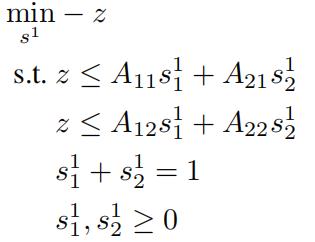
and show that this is a convex optimization problem (in s1).
(vii)What is the Lagrange dual of the problem in(vi)?
Observe that, interestingly, if we repeat parts (iv)-(vi) from the perspective of p2, we arrive at the same optimization as the dual of the analysis of p1 perspective. In game theory, this equivalence emerges as a result of duality is known as the minimax theorem, and is the reason why it does not matter if any of the players announce their optimal strategies a priori.
4 Predicting Restaurant-reviews via Perceptrons 代写机器学习
Download the review dataset restaurant reviews data.zip. This data set is comprised of reviews of restaurants in Pittsburgh; the label indicates whether or not the reviewer-assigned rating is at least four (on a five-point scale). The data are in CSV format (where the first line is the header); the first column is the label (label; 0 or 1), and the second column is the review text (text). The text has been processed to remove non-alphanumeric symbols and capitalization. The data has already been separated into training data reviews tr.csv and test data and reviews te.csv. The first challenge in dealing with text data is to come up with a reasonable “vectorial” repre-sentation of the data so that one can use standard machine learning classifiers with it.
Data-representations
In this problem, you will experiment with the following different data representations.
1.Unigram
In this representation, there is a feature for every word t, and the feature value associated with a word t in a document d is tf(t; d) := number of times word t appears in document d.
(tf is short for term frequency.)
2.Term frequency-inverse document frequency (tf-idf)
This is like the unigram representation, except the feature associated with a word t in a docu- ment d from a collection of documents D (e.g., training data) is
tf(t; d) × log10(idf(t; D)),
where tf(t; d) is as defined above, and
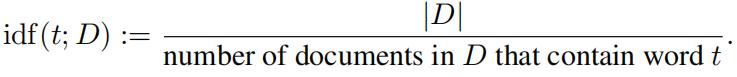
This representation puts more emphasis on rare words and less emphasis on common words. (There are many variants of tf-idf that are unfortunately all referred to by the same name.) 代写机器学习
Note: When you apply this representation to a new document (e.g., a document in the test set), you should still use the idf defined with respect to D. This, however, becomes problematic if a word t appears in a new document but did not appear in any document in D: in this case, idf(t; D) = D /0 = . It is not obvious what should be done in these cases. For this homework assignment, simply ignore words t that do not appear in any document in D.
3.Bigram representation.
In addition to the unigram features, there is a feature for every pair of words (t1, t2) (called a bigram), and the feature value associated with a bigram (t1, t2) in a given document d is tf((t1, t2); d) := number of times bigram (t1, t2) appears consecutively in document d.
In the sequence of words “a rose is a rose”, the bigrams that appear are: (a, rose), which appears twice; (rose, is); and (is, a).
For all the of these representations, ensure to do data “lifting”. 代写机器学习
Online Perceptron with online-to-batch conversion
Once can implement the Online Perceptron algorithm with the following online-to-batch con- version process.
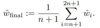
- Run Online Perceptron to make two passes through the training data. Before each pass, ran- domly shuffle the order of the training examples. Note that a total of 2n + 1 linear classifiers wˆ1,. . . , wˆ2n+1 are created during the run of the algorithm, where n is the number of training
- Returnthe linear classifier wˆftnal given by the simple average of the final n + 1 linear classi- fiers:
Recall that as Online Perceptron is making its pass through the training examples, it only updatesits weight vector in rounds in which it makes a prediction error. So, for example, if wˆ1 does not make a mistake in classifying the first training example, then wˆ2 = wˆ1. You can use this fact to keep the memory usage of your code relatively modest. 代写机器学习
(i)What are some potential issued with Unigram representation of textualdata?
(ii)Implementthe online Perceptron algorithm with online-to-batch You must submit your code to receive full credit.
(iii)Whichof the three representations give better predictive performance? As always, you should justify your answer with appropriate performance graphs demonstrating the superiority of one representation over the other. Example things to consider: you should evaluate how the classifier behaves on a holdout ‘test’ sample for various splits of the data; how does the training sample size affects the classification performance;
(iv)For the classifier based on the unigram representation, determine the 10 words that have the highest (i.e., most positive) weights; also determine the 10 words that have the lowest (i.e., most negative) weights.