代写机器学习作业 ECS708代写

ECS708 Machine Learning

Assignment 1 – Part 2: Logistic Regression and Neural Networks

代写机器学习作业 Fill out the sigmoid.py function by implementing the formula above. Now use the plot_sigmoid.py function to plot the sigmoid function.

Aim

The aim of this lab is to become familiar with Logistic Regression and Neural Networks.

1. Logistic Regression

From the root directory of the assignment’s code, navigate to the folder “assgn_1_part_2/1_logistic_regression”.

With logistic regression the values we want to predict are now discrete classes, not continuous variables. In other words, logistic regression is for classification tasks. In the binary classification problem we have classes 0 and 1, e.g. classifying email as spam or not spam based on words used in the email. The form of the hypothesis in logistic regression is a logistic/sigmoid function given by the formula below:

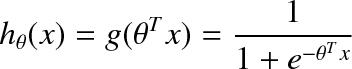
This is the form of the model. The cost function for logistic regression is

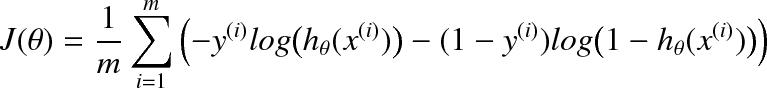
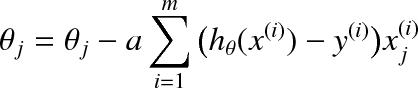
which when taking partial derivatives and putting these into the gradient descent update equation gives

Fill out the sigmoid.py function by implementing the formula above. Now use the plot_sigmoid.py function to plot the sigmoid function.

Task 1: Include in your report the relevant lines of code and the result of the using plot_sigmoid.py. [3 points]

The dataset we use is an exam score dataset with a 2-dimensional input space (for easy visualization) and a binary classification of whether the student was admitted or not. The data can be found in:”ex4x.dat” and “ex4y.dat”. The data has been loaded into the variables X and y. Additionally, the bias variable 1 has been added to each data point. Run plot_data.py to plot the data. Note that the data have been normalized, to enable the data to be more easily optimized.

Task 2. Plot the normalized data to see what it looks like. Plot also the data, without normalization. Enclose the plots in your report. [2 points]

1.1. Cost function and gradient for logistic regression 代写机器学习作业

Task 3. Modify the calculate_hypothesis.py function so that for a given dataset, theta and training example it returns the hypothesis. For example, for the dataset X=[[1,10,20],[1,20,30]] and for Theta = [0.5,0.6,0.7], the call to the function calculate_hypothesis(X,theta,0) will return: sigmoid(1 * 0.5 + 10 * 0.6 + 20 * 0.7)

The function should be able to handle datasets of any size. Enclose in your report the relevant lines of code. [5 points]

Task 4. Modify the line “cost = 0.0” in compute_cost.py so that we use our cost function:

To calculate a logarithm you can use np.log(x). Now run the file assgn1_ex1.py. Tune the learning rate, if necessary. What is the final cost found by the gradient descent algorithm? In your report include the modified code and the cost plot.

1.2. Draw the decision boundary

Task 5. Plot the decision boundary. This corresponds to the line where , which is the boundary line’s equation. To plot the line of the boundary, you’ll need two points of (x₁,x₂). Given a known value for x₁, you can find the value of x₂. Rearrange the equation in terms of x₂ to do that. Use the minimum and maximum values of x₁ as the known values, so that the boundary line that you’ll plot, will span across the whole axis of x₁. For these values of x₁, compute the values of x₂. Use the relevant plot_boundary function in assgn1_ex1.py and include the graph in your report. [5 points]

1.3. Non-linear features and overfitting 代写机器学习作业

We don’t always have access to the full dataset. In assgn1_ex2.py, the dataset has been split into a training set of 20 samples, and the rest samples have been assigned to the test set. This split has been done using the function return_test_set.py. Gradient descent is run on the training data (this means that the parameters are learned using only the training set and not the test set). After theta has been calculated, compute_cost() is called on both datasets (training and test set) and the error is printed, as well as graphs of the data and boundaries shown.

Task 6. Run the code of assgn1_ex2.py several times. In every execution, the data are shuffled randomly, so you’ll see different results. Report the costs found over the multiple runs. What is the general difference between the training and test cost? When does the training set generalize well? Demonstrate two splits with good and bad generalisation and put both graphs in your report.

In assgn1_ex3.py, instead of using just the 2D feature vector, incorporate the following non-linear features:

This results in a 5D input vector per data point, and so you must use 6 parameters θ. [2 points]

Task 7. Run logistic regression on this dataset. How does the error compare to the one found when using the original features (i.e. the error found in Task 4)? Include in your report the error and an explanation on what happens. [5 points] 代写机器学习作业

Task 8. In assgn1_ex4.py the data are split into a test set and a training set. Add your new features from the question above (assgn1_ex3.py). Modify the function gradient_descent_training.py to store the current cost for the training set and testing set. Store the cost of the training set to cost_vector_train and for the test set to cost_vector_test.

These arrays are passed to plot_cost_train_test.py, which will show the cost function of the training (in red) and test set (in blue). Experiment with different sizes of training and test set (remember that the total data size is 80) and show the effect of using sets of different sizes by saving the graphs and putting them in your report. In the file assgn1_ex5.py, add extra features (e.g. both a second-order and a third-order polynomial) and analyse the effect. What happens when the cost function of the training set goes down but that of the test set goes up? [5 points]

Task 9. With the aid of a diagram of the decision space, explain why a logistic regression unit cannot solve the XOR classification problem. [3 points]

2. Neural Network 代写机器学习作业

We will now perform backpropagation on a feedforward network to solve the XOR problem. The network will have 2 input neurons, 2 hidden neurons and one output neuron. There is also a bias on the hidden and output layer, e.g. with the following architecture:

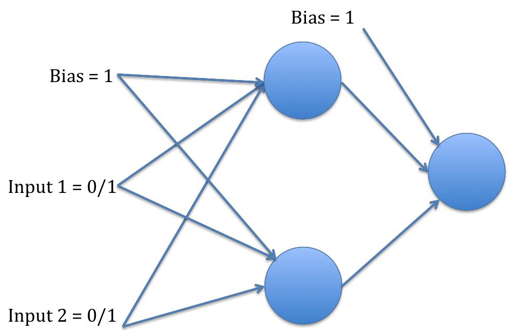
From the root directory of the assignment’s code, navigate to the folder “assgn_1_part_2/2_neural_network”.

Open the file xorExample.py. This is an example script that creates a neural network model as an object, initialized by using the class defined in NeuralNetwork.py.

Your first task is to modify the function sigmoid.py to use the sigmoid function that was implemented in the previous part, I.e. the logistic regression’s code.

The program works in the following way:

The arrays containing the input patterns (X) and the desired outputs (y) are created. These are passed to the train() function, that can be found in the file train_scripts.py. The train() function also takes as input arguments the number of hidden units desired (set to 2 for XOR), the number of iterations we should run the algorithm for, and the learning rate. 代写机器学习作业

In train() the neural network is created, and the main loop of the algorithm is executed. It works in the following way: For each iteration:

For each sample: forward_pass() backward_pass()

For each input pattern, we activate the network by feeding the input signal through the neurons. After this is completed, we compare the network’s output (i.e. the predictions), to the desired output (groundtruth labels), and update the weights using gradient descent.

Task 10. Implement backpropagation’s code, by filling the backward_pass() function, found in NeuralNetwork.py. Although XOR has only one output, your implementation should support outputs of any size. Do this following the steps below: [5 points]

Step 1. For each output, k, calculate the error delta:

where y_k is the response of the output neuron and t_k is the desired output (target). This error, , is multiplied by the derivative of the sigmoid function applied to the pre-sigmoided signal of the output neuron. The derivative of sigmoid, is implemented in the sigmoid_derivative.py function. Store each error in the output_deltas variable.

The first derivative, g’, of g(x) is: g’(x) = g(x) * (1-g(x))

As we have already calculated on the forward pass, in the code g’ is calculated using

Step 2. We now need to backpropagate this error to the hidden neurons. To accomplish this remember that:

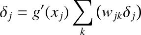
where δ_j is the error on the j-th hidden neuron, x_j is the value of the hidden neuron (before it has been passed through the sigmoid function), g′ is the derivative of the sigmoid function, δ_k is the error from the output neuron that we have stored in output_deltas, and w_kj is the weight from the hidden neuron j to the output neuron k. Once this has been calculated add δ_j to the array, hidden_deltas.

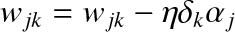
Step 3. We now need to update the output weights, i.e. the connections from the hidden neurons to the output neurons. This is accomplished using the formula:

where w_jk is the weight connecting the j-th hidden neuron to the k-th output neuron. a_j is the activity of the j-th hidden neuron (after it has been transformed by the sigmoid function), δ_k is the error from the output neuron stored in output_deltas and η is the learning rate.

Step 4. Finally we need to update the hidden weights, i.e. the connections from the hidden neurons to the inputs. Here, again we use this equation:

代写机器学习作业

where w_jk is the weight connecting the j-th input to the k-th hidden neuron. a_j is the j-th input, δ_k is the backpropagated error (i.e., hidden deltas) from the k-th hidden neuron and η is the learning rate.

2.1. Implement backpropagation on XOR 代写机器学习作业

Your task is to implement backpropagation and then run the file with different learning rates (loading from xorExample.py).

What learning rate do you find best? Include a graph of the error function in your report. Note that the backpropagation can get stuck in local optima. What are the outputs and error when it gets stuck?

Task 11. Change the training data in xor.m to implement a different logical function, such as NOR or AND. Plot the error function of a successful trial. [5 points]

2.2. Implement backpropagation on Iris

Now that you have implemented backpropagation we have built a powerful classifier. We will test this on the “Iris” dataset (http://en.wikipedia.org/wiki/Iris_flower_data_set), which is a benchmark problem for classifiers. It has four input features – sepal length, sepal width, petal length, and petal width – which are used to classify three different species of flower.

In irisExample.py, we have taken this dataset and split it 50-50 into a training and a test set.

Task 12. The Iris data set contains three different classes of data that we need to discriminate between. How would you accomplish this if we used a logistic regression unit? How is this scenario different, compared to the scenario of using a neural network? [5 points]

Task 13. Run irisExample.py using the following number of hidden neurons: 1, 2, 3, 5, 7, 10. The program will plot the costs of the training set (red) and test set (blue) at each iteration. What are the differences for each number of hidden neurons? Which number do you think is the best to use? How well do you think that we have generalized? [5 points] 代写机器学习作业

Write a report about what you have done, along with relevant plots. Save the solution in a folder with your ID. Create and submit a .zip that contains:

1)all of your codeand

2)a copy of your report. The report should be in .pdf format names aspdf a copy of your report. The report should be in .pdf format named as ml_lab1_part2_StudentID.pdf

合作平台：essay代写论文代写写手招聘英国留学生代写