
FNCE 435 – Empirical Finance
Assignment 3
代写实证金融课业 This assignment will explore data extraction from WRDS. The objective is to prepare the datasets that we will use in Module 4.
__________________________________________________________
This assignment will explore data extraction from WRDS. The objective is to prepare the datasets that we will use in Module 4. Jumping ahead to Module 4, we will replicate a study reported in CLM about market reactions to earnings announcements. The main figure of the study is shown below:
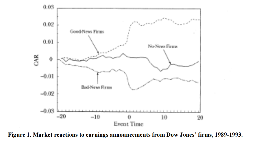
More specifically, we will look at market reactions to earnings announcements. Our sample will be quarterly earnings announcements for the 30 firms in the Dow Jones Index Average (DJIA), or simply Dow Jones index, between 1989 and 2003. (The results reported in CLM use the subsample of earnings from 1989 to 1993.)
The assignment is an example of an empirical examination that depends on data collection from many different sources. Here, the following data will be involved:
- The list of firms that have been part of the Dow Jones Index
- Data on earnings announcements for those firms
- Data on market expectations about earnings to be released
- Data on returns for the firms
- Data on returns for the market.
Let’s proceed step by step.
1. 代写实证金融课业
I collected for you the components of the Dow Jones index between 1989 and 2003. For each component, I show the PERMNO, CUSIP, and the period the company was part of the index (that is between INIT_DATE and END_DATE). This table is saved as a simple text file DJIA_DATA_1989_2003.txt, available on Canvas. Figure 1 shows the first few records of this text file (where the instructor took the liberty to add names to each column):
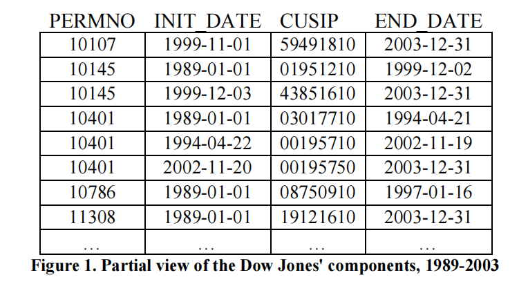
The first row shows that the company identified by the PERMNO=10107 was part of the index between November 1st, 1999 and December 31st, 2003. A second file, a SAS dataset named DJIA_NAMES_1989_2003, lists the name of each company; if you print that file you will see that PERMNO=10107 refers to Microsoft Corp. 代写实证金融课业
The next two rows shows records for the same firm—the one with PERMNO=10145 (you can check that its name is Honeywell International Inc). Two records are necessary because there was a change in the CUSIP for that firm: between January 1st, 1989 and December 2nd, 1999 its CUSIP was “019521210”, while between December 3rd, 1999 and December 31st, 2003 its CUSIP was “43851610”. This distinction is important because at times we will collect data based on PERMNO, at times based on CUSIP.
Read this data into a SAS code. You can either read the file directly or copy and paste the contents of the file into your code and use the DATALINES statement. Force the CUSIP variable to be of the character datatype. Also, make sure you read the dates correctly by using the proper informat. (To recognize a date written as YYYY-MM-DD, use the informat “yymmdd10.”) After reading the dataset into your SAS code, print it to make sure the import worked.
2. 代写实证金融课业
Now let’s work on the earnings data. Earnings data is collected by the IBES database in WRDS, whose physical location is ‘/wrds/ibes/sasdata’. The first info we will collect refer to the quarterly earnings announcements. The IBES dataset ACTU_EPSUS contains such information. Create a library in your SAS code with a logical reference to the IBES directory and proceed with a PROC CONTENTS on the ACTU_EPSUS dataset. Take a look at the output. In particular, notice how many records the dataset has.
You will see a bunch of variables. What you won’t see is a PERMNO variable. Instead, the identifiers for a company in IBES are CUSIP and OFTIC (the official ticker for the firm). Fortunately, you already have the CUSIP for the Dow Jones components, so you can search for a company’s earnings using its CUSIP.
a) 代写实证金融课业
Start the data collection by obtaining data from ACTU_EPSUS for the sample of firms collected in step 1. That is, combine the ACTU_EPSUS with your Dow Jones file based on the variable CUSIP, so that only observations from the ACTU_EPSUS that are also on the Dow Jones file are kept.
You should try a PROC SQL with a CREATE command to create such a table (dataset), similar to what we have done in Section 5 of Module 3. The PROC SQL should bring all variables from each dataset. The WHERE condition should match the CUSIP variable from each dataset. Look at the log file to note how many records were created in this new dataset.
b) 代写实证金融课业
The final earnings dataset should have 1,800 observations (30 components of Dow Jones each quarter times 60 quarters). As of now, we have many more observations. This is because we did not put any other restriction on the data collection. For example, for PERMNO=10145 we are bringing many more earnings (annual, quarterly, before 1989, after 2003, etc) than the 60 quarters we need from 1989 thru 2003. Our next step is to filter out the data we do not need. Here they are:
- The variable PENDS from ACTU_EPSUS indicates the quarter of the earnings observation. It is a variable stored as a date, more specifically, the last date of the calendar quarter to which that earnings data refers to. For example, earnings for the 2nd quarter of 2000, which finishes in the end of June, will have PENDS= 30JUN2000”d. Thus, if I need the earnings data for the year 2000, I would use a restriction in my data collection as in “01JAN2000”d<=PENDS<=”31DEC2000”d. For our sample, Use the initial and end date from the Dow Jones table to restrict the quarters you are accessing; that is, you will need to write a filter such as INIT_DATE<=PENDS<=END_DATE. 代写实证金融课业
- The variable PDICITY from ACTU_EPSUS indicates periodicity of the earnings data. Companies release both quarterly (PDICITY=”QTR”) and annual (PDICITY=”ANN”) earnings. Since our study uses quarterly earnings, you will need to restrict your data collection to observations with PDICITY=”QTR”.
- Earnings data includes information on various earnings measures, which are collected in different observations, as recorded in the variable MEASURE from ACTU_EPSUS: earnings per share (MEASURE=”EPS”), cash flows per share (MEASURE=”CFS”), etc. We will look at earnings per share only, thus restrict your data collection to observations with MEASURE=”EPS”.
Apply the three restrictions above over the dataset you created in step a). 代写实证金融课业
Use a WHERE condition in a DATA step. For example, if the dataset from a) is named D, create a dataset E as
data e;
set d
where <restrictions>;
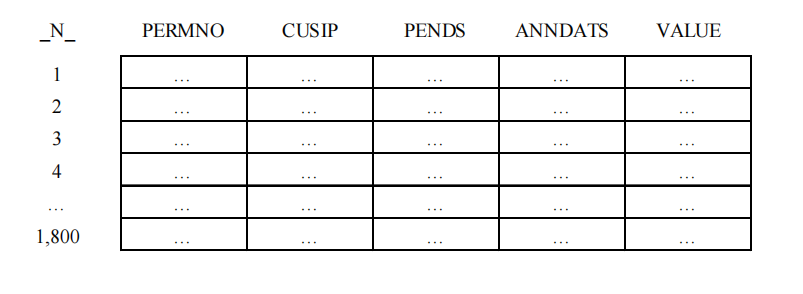
Verify that your new dataset ends up with 1,800 observations. The additional variables you will need—besides the ones identifying the earnings (PERMNO, CUSIP, and PENDS)— are: the exact date of the announcement (ANNDATS from ACTU_EPSUS) and the actual value of the earnings that were announced (VALUE from ACTU_EPSUS). Thus, keep in your dataset only these variables. The dataset you want to create has the following format:
3.
IBES also records the output of sell-side analysts. In particular, IBES records detailed earnings forecasts by sell-side analysts. Besides detailed data, IBES records summary statistics on these forecasts, such as the mean forecast by these analysts. We will need these mean forecasts as a proxy for the market expectation on upcoming earnings.
Let’s say that we wanted to know what was the market expectation, as of June 30, 2000, about the 2nd quarter of 2000’s earnings for IBM. This 2nd quarter’s earnings would be released sometime after June 30, 2000 (which is the end of the 2nd quarter). All we need to do is to look for the summary statistics on earnings forecasts for IBM around that specific date. 代写实证金融课业
Data on summary statistics on earnings forecasts is stored in the STATSUMU_EPSUS dataset of the IBES database. Please use the PROC CONTENTS on this dataset. An observation from this dataset is identified by the firm’s identifier (OFTIC, CUSIP), by the fiscal quarter it refers to (FPEDATS, equivalent to the PENDS variable in the ACTU_EPSUS dataset), by the type of the earnings number (FISCALP, equivalent to the PDICITY variable in the ACTU_EPSUS dataset), by the measure (MEASURE, as in the ACTU_EPSUS dataset), and by the date the summary statistics was computed (STATPERS variable).
Thus, in our example above for IBM, I would look for the observations in the STATSUMU_EPSUS dataset that attend to the following clause:
cusip=”45920010” and measure=”EPS” and
fiscalp=”QTR” and fpedats=”30JUN2000”d and
statpers<=”30JUN2000”d;
a) 代写实证金融课业
Please try to collect the summary statistics data for IBM according to the above conditions. Please print these observations. How many such observations are available?
You will notice that the clause above reads all summary statistics that were generated for that quarter for IBM, that is, potentially one generated in March 2000, another in April 2000, etc. An additional step would be to clean up the data to keep the one that is closest to June 30, 2000, that is, simply the latest such observation. In this case, it would be the observation with the STATPERS closest to, but before, June 30, 2000. What is the date (STATPERS) of this observation?
b) 代写实证金融课业
Now, for the sample of earnings data you obtained in step 2, collect summarystatistics on earnings forecasts that are available before the end of the fiscal quarter.Here you should use a PROC SQL so that you can match the summary stats dataset with the earnings dataset, based on CUSIP and the dates. The search condition should include a restriction that the STATPERS in the summary stats dataset is smaller than or equal to the PENDS variable in the earnings dataset, or STATPERS≤PENDS.
The next step is to keep only the latest summary statistics for each quarter. The main variable you will need from the STATSUMU_EPSUS dataset is MEANEST (the average earnings forecast).
Now, a hint on how you can “keep only the latest summary statistics for each quarter.” There are many ways to accomplish this, but here is one.
Suppose you have a dataset D with all summary statistics for a quarter. 代写实证金融课业
Each observation is uniquely identified by the variables PERMNO, PENDS, and STATPERS. In database parlance, we say that the combination of (PERMNO, PENDS, STATPERS) is a primary key for this dataset.
The idea is to use the NODUPKEYS clause in a PROC SORT; the clause keeps only one observation per set of variables identified in the BY clause. The code should be written as shown below:
proc sort data=d;
      by permno pends descending statpers;

proc sort data=d nodupkeys;
      by permno pends;
This code sorts the D dataset by PERMNO, PENDS, then by the date the summary statistics was taken. The DESCENDING clause tells to sort by STATPERS in a descending fashion—so that the most recent (or latest) date of STATPERS appears first for each value of PERMNO and PENDS. The 2nd PROC SORT keeps only one observation per pair of PERMNO and PENDS, but since the dataset is already sorted by STATPERS (in an descending fashion), only the latest summary statistics is kept for each quarter.
4. 代写实证金融课业
Let’s look inside the data. Read your datasets and extract the following information. For IBM (PERMNO=12490) and the quarter ending in June 30, 2000, what was the date of its earnings announcement? Which value for the earnings was announced at the time? What was the market expectation (mean estimate) for the upcoming earnings? When was that estimate produced? Was the newly announced earnings a positive or negative surprise with respect to what sell-side analysts were anticipating?
5.
Combine the data on earnings announcements and summary statistics in one single dataset. This final dataset should be named EARNINGS_1989_2003, and contain the following variables: PERMNO, PENDS, ANNDATS, VALUE, and MEANEST.
Download this dataset to your SAS library in the Windows environment. Make sure that this dataset contains again 1800 observations. That is, the format of your dataset should be:
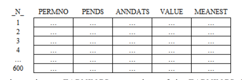
Please create also a dataset EARNINGS as a subset of the EARNINGS_1989_2003
containing only the earnings with PENDS between January 1st, 1989 and December 31st, 1993. This EARNINGS dataset will be used in class to replicate the results from CLM. This dataset should have 600 records.
6.
You will also need data on returns. For the sample described in step 1, collect the variables DATE and RET from the dataset DSF from the CRSP database (whose physical location is the directory ‘/wrds/crsp/sasdata/a_stock’).
Be careful here: the DSF dataset has return data on all public companies since 1926—you need returns only the sample of companies belonging to the DJIA over the period 1989- 2003. In other words, you should bring return data from DSF only for the firms that are also on the Dow Jones file you obtained in step 1). The primary identifier of a firm in DSF is PERMNO, not CUSIP. You thus should employ a PROC SQL with its WHERE clause matching PERMNOs from both files. 代写实证金融课业
Another restriction on which return data to bring is that returns should be collected in the period 01/01/1988 through 12/31/2004. (This is because we need data on early 1994 to analyze the earnings announcements from the last fiscal quarter of 1993.)
Thus, create a dataset called RETURNS, with the following variables: PERMNO, DATE, and RET. The basic dataset should look like:
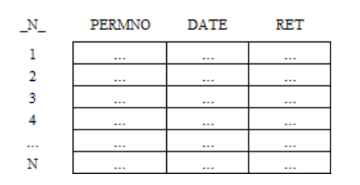
Hint: there are 40 different PERMNOs in the Dow Jones dataset 17 years of daily returns, we should expect the number of observations N in the table above to be around 170,000 observations (each year has about 252 trading days, thus a first guess on the number of observations is 40*17*252=171,360). You can check using PROC CONTENTS if this guess is Ok.
7. 代写实证金融课业
Download index returns (variable VWRETD) from the dataset DSIX (whose physical location is the directory ‘/wrds/crsp/sasdata/a_indexes’). Use the same period adopted in the previous step, 01/01/1988 through 12/31/2004. The final dataset should be named MARKET_RETURNS, and have the following variables: DATE (corresponding to the variable CALDT in the DSIX dataset) and VWRETD. The table is like:
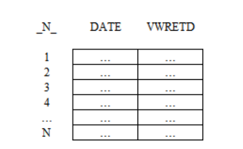
with a guess that N=17*252=4,284.
8.
Finally, some test. Your earnings dataset has the VALUE and MEANEST measures. For each observations in the earnings dataset, define a variable SURPRISE as VALUE minus MEANEST, then test the null hypothesis that analysts do a very good job of predicting earnings, that is, that surprise is on average zero,
H0: E(SURPRISE) = 0
Ha: E(SURPRISE) ≠ 0
Compute the t statistic and the p-value, test the hypothesis (with a significance level of 5%), then define a 95% confidence interval for the SURPRISE measure. Discuss the results.

更多代写:新西兰程序代写 gre?proctoru代考 英国心理学代写 compare and contrast essay怎么写 memo范文 斯坦福大学申请代写
