
Re-analyze the data
Name
Professor
Institution
Course
Date
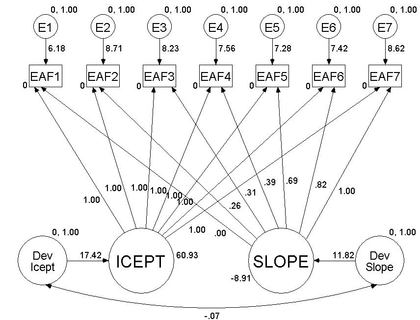
代写分析数据essay I do not agree with the authors conclusion and analyses because the models are both recursive and they have no feedback loops.
AMOS model 代写分析数据essay
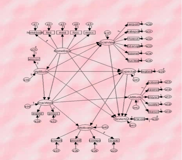
Author’s conclusion and analyses:
I do not agree with the authors conclusion and analyses because the models are both recursive and they have no feedback loops. Some of the arrows share some basin features seen in recursive models. These factors tend to simplify the statistical demands for the actual analyses associated with them. Their errors or the degree of disturbance is uncorrelated while at the same time, the causal effects are all unidirectional
| Unstandardized Estimate | Standardized Estimates | ||
| Aptitude | 0.002 | 0.001 | |
| Aptitude | 0.021 | 0.002 | |
| Aptitude | 0.04 | 0.005 | |
| Prac-Work | 3.41 | 0.357 | |
| Home-Back | 0.161 | 0.044 | |
| Expectat | 0.043 | 0.007 | |
| ScieView | 2.114 | 0.227 | |
| Expectat | 0.895 | 0.113 | |
| Aptitude | 0.647 | 0.03 | |
| Attitude | 2.356 | 0.299 | |
| 代写分析数据essay | |||
Fit indices generated from an AMOS program
| Model NPAR CMIN DF P CMIN/DF | ||||||||
| ———————————————————————— | ||||||||
| Final model 128 7613.772 522 0.000 14.586 | ||||||||
| Saturated model 650 0.000 0 | ||||||||
| Independence model 50 65261.700 600 0.000 108.770 | ||||||||
| ———————————————————————— | ||||||||
| ———————————————————————— | ||||||||
| Model RMR GFI AGFI PGFI | ||||||||
| ———————————————————————— | ||||||||
| Final model 0.145 0.922 0.903 0.741 | ||||||||
| Saturated model 0.000 1.000 | ||||||||
| Independence model 1.325 0.424 0.376 0.391 | ||||||||
| ———————————————————————— | ||||||||
| 代写分析数据essay | ||||||||
| ———————————————————————— | ||||||||
| Model DELTA IFI RH02 TLI CFI | ||||||||
| ———————————————————————— | ||||||||
| Final model 0.890 0.874 0.890 | ||||||||
| Saturated model 1.000 1.000 | ||||||||
| Independence model 0.000 0.000 0.000 | ||||||||
| ———————————————————————— | ||||||||
| ———————————————————————— | ||||||||
| Model RMSEA LO 90 HI 90 PCLOSE | ||||||||
| ———————————————————————— | ||||||||
| Final model 0.043 0.042 0.044 1.000 | ||||||||
| Independence model 0.121 0.120 0.122 0.000 | ||||||||
Measurement model by use of LISREL: Here is the correlation matrix:
| X1 | X2 | X3 | X4 | X5 | |
| X1 | 1.00 | ||||
| X2 | 0.28 | 1.00 | |||
| X3 | 0.16 | 0.10 | 1.00 | ||
| X4 | 0.03 | 0.04 | 0.52 | 1.00 | |
| X5 | 0.15 | 0.05 | 0.59 | 0.36 | 1.00 |

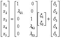
The formulas and the equations are as bellow:
X = Λx ξ + δ
x1 = 1*ξ1 + 0*ξ2 + δ1
x2 = l21*ξ1 + 0*ξ2 + δ2
x3 = 0*ξ1 + 1*ξ2 + δ3
x4 = 0*ξ1 + l42*ξ2 + δ4
x5 = 0*ξ1 + l52*ξ2 + δ5
Other matrices:
δ (5×5 matrix of variance and covariance of the measurement errors δ ) – Measurement error varies but fails to covary. Therefore, the matrix is made to be diagonal and free – this necessitates the use of LISREL default (Muller, Judd, &,Yzerbyt, 2005). 代写分析数据essay
Φ (2×2 matrix of the variance and covariance of the exogenous variable ξ) –With the pure measurement models, it is advisable to allow the latent variables to covary and connect all by the double-headed arrows. Consequently, estimate all the elements of the matrix — symmetric, free.
DA NI=5 NO=100 MA=KM
LA
SCOREA, SCOREB victimization, unilateral bids, exclusion
1.00
0.28 1.00
0.16 0.10 1.00
0.03 0.04 0.53 1.01
0.15 0.05 0.52 0.34 1.001
MO NX=5 NK=2 LX=FU, FI
LK
Victimization,
FR LX 3 1 LX 52 LX 5 2
VA 1.0 LX2 1 LX 4 2
PD
OU
Output:
DA NI=5 NO=100 MA=KM
Amount of Input Variables 5
Amount of Y – Variables 0
Amount of X – Variables 5
Amount of ET – Variables 0
Amount of KS – Variables 2
Amount of Observations 100
DA NI=5 NO=100 MA=KM
Correlation Matrix
Score A. Score B. Victimization, unilateral bids, exclusion
——– ——– ——– ——– ——–
SCORE1 1.00
score2 0.28 1.00
Victimization, 0.16 0.10 1.00
Unilateral bids, 0.03 0.04 0.52 1.00
Exclusion 0.15 0.05 0.59 0.36 1.00
DA NI=5 NO=100 MA=KM
Parameter Specifications
β-X
ABILITY PEER
——– ——–
SCORE1 0 0
SCORE2 1 0
Victimization, 0 0
Unilateral bids 0 2
Exclusion 0 3
phi
Victimization, unilateral bids
——– ——–
Unilateral bids 4
Victimization, 5 6
Theta-Delta
SCOREA SCORE B Victimization unilateral bids Exclusion
——– ——– ——– ——– ——–
7 8 9 10 11
DA NI=5 NO=100 MA=KM
Number of Iterations = 10
LISREL Estimates (Maximum Likelihood) 代写分析数据essay
LAMBDA-X
ABILITY PEER
——– ——–
SCORE1 1.00 – –
SCORE2 0.60 – –
(0.63)
0.95
SEAT – – 1.00
SCHOOL – – 0.60
(0.14)
4.24
PLAY – – 0.69
(0.15)
4.52
PHI
ABILITY PEER
——– ——–
ABILITY 0.47
(0.50)
0.92
PEER 0.16 0.86
(0.10) (0.21)
1.57 4.03
Theta-delta
scoreA scoreB seat school play
——– ——– ——– ——– ——–
0.53 0.83 0.18 0.61 0.29
(0.80) (0.21) (0.26) (0.21) (0.21)
1.0 3.70 0.75 6.12 5.33
Squared Multiple Correlations for X – Variables
ScoreA Score B SEAT SCHOOL PLAY
——– ——– ——– ——– ——–
0.42 0.17 0.76 0.41 0.21
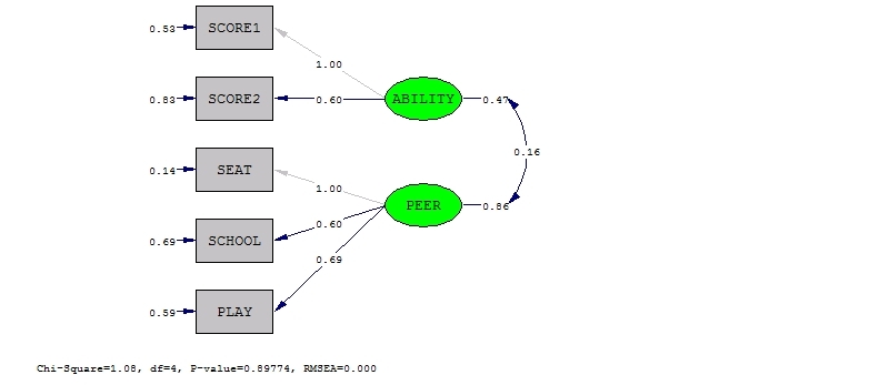
Goodness of Fit Statistics 代写分析数据essay
Degrees of Freedom = 4
Minimum Fit Function Chi-Square = 1.09 (P = 0.90)
Normal Theory Weighted Least Squares Chi-Square = 1.08 (P = 0.90)
Estimated Non-centrality Parameter = 0.0
90 Percent Confidence Interval for NCP = (0.0; 3.72)
Minimum Fit Function Value = 0.011
Population Discrepancy Function Value (F0) = 0.0 代写分析数据essay
90 Percent Confidence Interval for F0 = (0.0; 0.017)
Root Mean Square Error of Approximation (RMSEA) = 0.0
95 Percent Confidence Interval for RMSEA = (0.0; 0.066)
P-Value for Test of Close Fit (RMSEA < 0.05) = 0.93
Expected Cross-Validation Index (ECVI) = 0.26
90 Percent Confidence Interval for ECVI = (0.26; 0.28)
ECVI for Saturated Model: = 0.30
ECVI for Independence Model: = 0.99
Chi-Square for Independence Model with 10 Degrees of Freedom = 88.07
Independence AIC = 98.07
Model AIC = 23.08
Saturated AIC = 30.00
Independence CAIC = 126.10
Model CAIC = 62.74
Saturated CAIC = 84.08
Normed Fit Index (NFI) = 4.99
Non-Normed Fit Index (NNFI) = 1.04
Parsimony Normed Fit Index (PNFI) = 0.42
Comparative Fit Index (CFI) = 1.00
Incremental Fit Index (IFI) = 1.33
Relative Fit Index (RFI) = 0.57
Critical N (CN) = 123.77
Root Mean Square Residual (RMR) = 0.011
Standardized RMR = 0.031
Goodness of Fit Index = 1.00
Adjusted Goodness of Fit Index (AEFI) = 0.48
Parsimony Goodness of Fit Index (PGEI) = 0.57
Correlation is a measure of the association between two variables.
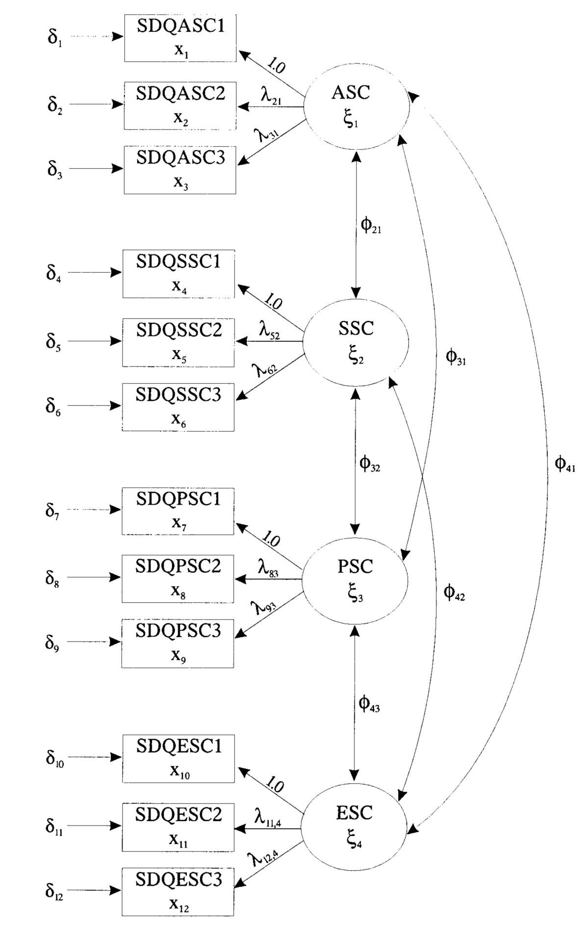
(a) Run the 4-factor model displayed in Figure 1 9 (give your AMOS diagram with unstandardized coefficients)
Note: Use BANH1, SDEP, BANX1 and SSOM as reference indicators for their respective factors
(b) Run the 3-factor model andgive your AMOS diagram with unstandardized coefficients)
Note: Use BANH1, SDEP and SSOM as reference indicators for their respective factors
Run the second order factor model displayed in Figure 4 (give your AMOS diagram with unstandardized coefficients)
(c) Test whether the unstandardized factor loadings and error terms for the first order NonSpecific Depression and Anhedonia factors are equal (as reported on p. 467) – give details of your chi-square difference tests.
Unstandardized factor loadings and error terms for the first order NonSpecific Depression and Anhedonia factors not equal and their give details of your chi-square difference tests are as shown below:
Scaling factor for the whole model = 0.916, and for the quadratic = 1.21; the overall linear model parameters that are estimated is= 5, while that of the quadratic model is 11 paramters
The unstandardised factor ladings and errors for the original order non specific anxiety and and somaticmarousal factors are not equeal. The detail of the chi-square difference tests are: 代写分析数据essay
Scaling factor for the whole model = 1.36, and for the quadratic = 1.128; the overall linear model parameters that are estimated is9, while that of the quadratic model is 10 paramters).
(e) (Hard question!) Reproduce the variance decomposition for the Philadelphia outpatient sample reported in Table 4.
(f) Comment on the paper’s conclusions.
3.What are the advantages and disadvantages of item parceling? 代写分析数据essay
Parceling is a statistical practice that involves combining data or items into small subsets or groups. This may require the data manager to putting the data into a single parcel, split the items into odd or even groups, and balance the discrimination of items such as through item-to-construct balance. Random selection of a specific number of items is also possible as well as creating multiple parcels, or grouping the data into similar factors loadings such as contiguity (Nasser, & Takahashi, 2003; Imai, Keele, and Yamamoto, 2010).
Advantages
Parceling has a number of advantages some of the main advantages include the empirical advantages.
Increase reliability-The most outstanding advantage is the ability to increase the reliability of the data used. With parceling, the data become more reliable because the data undergoes inspection and triangulation.
Achieving normality- for the data to have a normal distribution, the data manager can parcel the items.
Adapting to small sample sizes-it is easy to work with small sample sizes than with large sample, therefore if items are grouped according to their sample sizes; they become easy to manage as the data specialist split the items according to their nature such as odd, even, discrete or continuous. 代写分析数据essay
Reduce idiosyncrasy that influences the individual items- individual items are not easily influenced by common features in an item set.
simplifying interpretation: interpreting data sets is very difficult, but parceled data is easy to analyze and integrate
Better model fit- model fit is easy to obtain with parceled data than with lose data.
Advantages
According to Schau, Stevens, Dauphinee, & Del Vecchio, (1995), parceling also has a host of disadvantages that may result into disastrous conclusions. Some of the main disadvantages include misspecified models that fit more appropriately than specified item. Additionally, parceling may also obscure unmodeled features. However, Nasser, & Takahashi, (2003), notes that, the most outstanding disadvantage is that parceling can Cause a decrease in the overall convergence to an appropriate solution as compared to the individual indicators
Reference 代写分析数据essay
Schau, C., Stevens, J., Dauphinee, T. L., & Del Vecchio, A. (1995). The development and validation of the Survey of Attitudes toward Statistics. Educational and Psychological Measurement, 55, 868–875.
Nasser, F. & Takahashi, T.(2003). The effect of using item parcels on ad hoc goodness-of-fit indexes in confirmatory factor analysis: An example using Sarason’s Reactions to Tests. Applied Measurement in Education, 16, 75–97.
Thompson, B., & Melancon, J. G. (1996). Using item “Testlest”/“Parcels” in confirmatory factor analysis: An example using the PPSDQ-78. (ERIC Document No. ED 404 349)
Imai, K., Keele, L., and Yamamoto, T., (2010). Identification, inference, and sensitivity analysis for causal mediation effects. Statistical Science, 25(1):51–71, 2010.
Muller, D., Judd, C. M., Yzerbyt, V. Y. (2005). When moderation is mediated and mediation is moderated. Journal of Personality and Social Psychology, 89(6), 852–863.