Physics 307 Homework DEMO
The answer set in here due date:Thursday,18,October,at 5PM
Q 1 answer
Suppose there are N+1 nodes in one string, and its unstretched length is and stretched length is L. Then we can easily get the k by Hooke’s-law:
And we know that the linear mass density of the unstretched string can be expressed as:
Also, the unstretched distance between two connected nodes are:
Considering the stiffness’s definition, the relationship between k and stiffness can be expressed as:
Q 2 answer
To simulate the vibrations of a stretched string of uniform density and elasticity, we can build a 2-dimention matrix to storage the conditions of different nodes in different time. The row stands for the time and lines stands for the order of nodes . By introducing the leapfrog solver, the state of node in next step is determined by the state now, as shown in the next equation:
The C code is shown down here:
#include <stdio.h>

#include <math.h>

int main()

{ int N=50,i=0,j=0;

double dt=0.00001,tmax=0.8,L0=0.3,u=30;

    double r0=L0/N,k=u/L0,density=1/30,m=density*L0/N,T=10;

int Nmax=tmax/dt;

double r1,r2,dx,xc,sigma,A;

    double x[Nmax][N+1],y[Nmax][N+1],vx[Nmax][N+1],vy[Nmax][N+1],t[Nmax],E[Nmax] ;

dx=(T/k+L0)/N;

    xc=(T/k+L0)/2;

    sigma=1;

    A=0.1;

    for (i=0;i<(N+1);)

{

x[0][i]=i*dx;

vx[0][i]=0;

y[0][i]=A*(exp((-x[1][i]-xc)*(-x[1][i]-xc)/sigma*sigma)-exp(-xc*xc /sigma*sigma));

vy[0][i]=0;

}

    for (i=0;i<(Nmax);)

{

x[i][N]=(T/k+L0);

x[i][0]=0;

vx[i][N]=0;

vx[i][0]=0;

y[i][N]=0;

y[i][0]=0;

vy[i][N]=0;

vy[i][0]=0;

}


for (i = 0; i<(Nmax-2);)

{

for (j = 1; j<(N-1);)

{ x[i+1][j]=x[i][j]+vx[i][j]*dt/2;

     y[i+1][j]=y[i][j]+vy[i][j]*dt/2;

     r1=sqrt((x[i][j]-x[i][j-1])*(x[i][j]-x[i][j-1])+(y[i][ j]-y[i][j-1])*(y[i][j]-y[i][j-1]));

     r2=sqrt((x[i][j]-x[i][j+1])*(x[i][j]-x[i][j+1])+(y[i][ j]-y[i][j+1])*(y[i][j]-y[i][j+1]));

     vx[i+1][j]=vx[i][j]-(x[i][j]-x[i][j-1])*(1-r0/r1)*k*dt/ m-(x[i][j]-x[i][j+1])*(1-r0/r2)*k*dt/m;

     vy[i+1][j]=vy[i][j]-(y[i][j]-y[i][j-1])*(1-r0/r1)*k*dt/ m-(y[i][j]-y[i][j+1])*(1-r0/r2)*k*dt/m;

     x[i+1][j]=x[i+1][j]+vx[i+1][j]*dt/2;

     y[i+1][j]=y[i+1][j]+vy[i+1][j]*dt/2;

     t[i+1]=t[i]+dt;

     E[i]=E[i]+m*(vx[i][j]*vx[i][j]+vy[i][j]*vy[i][j])/2+k* (r1-r0)*(r1-r0);

 i=i+1;

}

}


for (i = 0; i<(Nmax-2); i++)

     printf("%lf %lf \n",x[i][5], y[i][5]);

printf("\n");


}
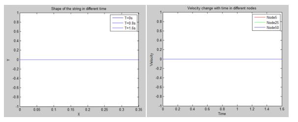
Q 3.Applying a tension T to the string, the length of the string is changed to (L0+T/k). Then the position for each node should be changed, too. In the simulation, the time step is set as 1e-5s and the total simulation time is set as 1.6s. The original length of the string is 0.3m and the number of the nodes in total is 100. The stiffness is chosen as 60 and the linear density is 1/30, which means the mass of each mode is 1e-4 Kg. The figure in the left shows the shape of the string in different time. We take t=0s, t=0.8s and t=1.6s as three examples, which clearly shows that the shape doesn’ t change in the whole simulated time. To better demonstrate the string doesn’t move, we also plot the relationship between velocity and time for three different nodes. The result is shown in the right figure. From this figure,the velocity of three nodes in the string remains zero.
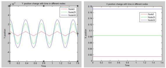
Q 4. Taking the Gaussian deformation as an example, the A is 0.1, sigma is 1 and xc is the center of the string. Then the center of the string has the largest deformation and the position of these nodes is symmetric. Firstly, we plot the x and y position VS time for three nodes, which is shown down here. It is clearly that each node has a periodic deformation in y but remain the same position in x. This means the deformation is horizontal. For Node 25 and Node 50, the relationship between deformation and time seems like trigonometric function while for Node 5 it is more like a linear relationship. This is because for Node 5, the deformation is small and the speed can be regarded as a constant.
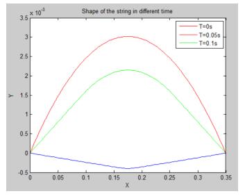
Also we plot the shape of the string in different time, which can see the deformation process more clearly. In this figure, the curve stands for the string, we can see that at T=0s. it is at the original condition, which is a Gaussian deformation. As time goes by, the string shrink and the deformation become smaller but the speed increases, this is because the transfer between kinetic energy and potential energy.
Q 5. In a guitar or violin, the sound is form the vibration of strings. We know that there are three important properties of sound, loudness, frequency and timbre. The loudness is determined by the deformation amplitude and the timbre is determined by the material itself, which are directly can be understood. As for the frequency, which can be calculated through the vibration period, it is quite complicated and interesting.
Firstly, we discuss its relationship with external tension T. By changing the external tension T from 5 to 50N, we can plot the figure. It shows that by changing the external tension, the frequency of the sound can be easily changed, which is quite similar to the process of tuning the real piano.
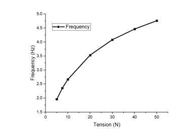
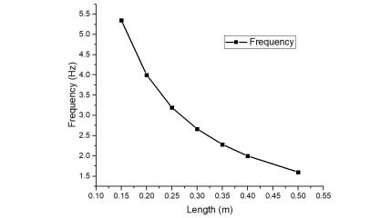
Except for changing the tension of the string, when we play the piano, the position of the finger is also important, which means the length of the string can also have important impact on the sound. Here is the simulated result that we fix the tension as 10N and vary its length from 0.15m to 0.5m:
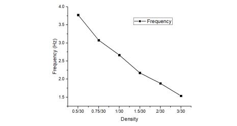
Also, the mass for each node is important, which corresponds to the linear density of the string. And we fix the tension at 10N and length at 0,3m, then the relationship is shown below:
Q 6. The total energy has an equation as described as:
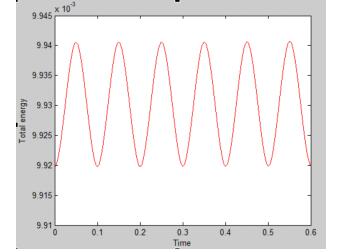
Then we add the integration for total energy in the code and plot its relationship with time. As the figure shows, the total energy nearly conserves as a constant. The vibration is originated from the finite time step and space step while the amplitude of the noise actually is small and can be ignored.
Then we add the integration for total energy in the code and plot its relationship with time. As the figure shows, the total energy nearly conserves as a constant. The vibration is originated from the finite time step and space step while the amplitude of the noise actually is small and can be ignored.
