ACS61010 Optimal Control
Optimal Control代写 You should not discuss the assignment with other students and should not work together in completing the assignment.
Coursework
Assignment weighting
15%
Assignment released
Monday, 20 March (Week 7)
Assignment due
Sunday, 7 May, 23:59 (Week 10)
Penalties for late submission
Late submissions will incur a 5% reduction in the mark for every working day (or part thereof) that the assignment is late and a mark of zero for submission more than 5 working days late.
How to submit Optimal Control代写
- Use the “Coursework (written solution)” link on Blackboard to submit your written solution.
- Use the “Coursework (MATLAB)” link on Blackboard to submit your Matlab files in a single ZIP archive.
Feedback
You will receive feedback via Blackboard. The intention is to provide feedback two weeks after the submission deadline, but this may be changed due to extenuating circumstances forms submitted by other students.
Unfair means
The assignment should be completed individually. You should not discuss the assignment with other students and should not work together in completing the assignment. The assignment must be wholly your own work. References must be provided to any other work that is used as part of this assignment. Any suspicions of the use of unfair means will be investigated and may lead to penalties.See https://www.sheffield.ac.uk/ssid/unfair-means/index for guidance.
Extenuating circumstances Optimal Control代写
If you have medical or personal circumstances that cause you to be unable to submit this assignment on time or that may have affected your performance, please, complete an extenuating circumstances form and submit it to acse-support@sheffield.ac.uk along with the evidence of the circumstances. See https://www.sheffield.ac.uk/ssid/forms/circs for more information.
MATLAB help
- Matlab Onramp
- Solving Ordinary Differential Equations with Matlab
- Solving Boundary Value Problems with Matlab
- Tutorial on solving BVPs with BVP4C

Assignment briefing
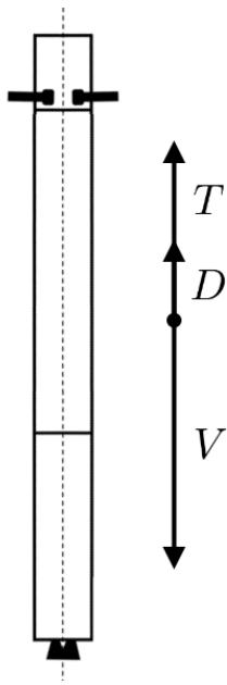
Problem 1. Consider the optimal landing of a rocket booster con-sidered in Lecture 1. In Problem Set 1, we saw that, if the rocket is oriented vertically, the model becomes
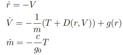
where
- r is the radial distance from the Earth’s centre;
- V is the speed;
- m is the rocket mass;
- T ∈ [0, TM] is the thrust magnitude (control);
- D(r, V ) is the drag force (a function of r and V );
- g(r) is the gravitational acceleration at r;
- g0 is the gravitational acceleration at R⊕ (Earth radius);
- c is a constant that depends on the engine type.
Assume that the booster’s speed is 1100 km/h when its altitude (the distance to the surface of Earth) is 5 km. The mass of an empty booster is 25,600 kg and it has 2,500 kg of fuel.
a.Show that the optimal control for the minimum-time problem is “bang-bang”. Write down the costate equations and boundary conditions.[10 marks]
b.Show that the optimal control for the minimum-fuel problem is “bang-bang”. Write down the costate equations and boundary conditions.[10 marks]
c.The last two equations describing the booster dynamics imply

Assuming that D(r, V ) < mg(r) (the gravity is stronger than the drag), show that the con-sumed fuel is a monotone increasing function of the final time. (Hint: You need to integrate both sides from 0 to tf and use V (tf ) = 0.) What does this observation allow us to conclude about the relation between the solutions of the minimum-time and minimum-fuel problems? [15 marks]
d.The calculations above suggest that the optimal minimum-time control has the form
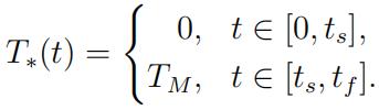
Write a Matlab program that solves the state equations for given ts and tf . Use this program to find the optimal values of ts and tf. Plot the optimal state.
When solving the state equations, assume that the drag force is given by
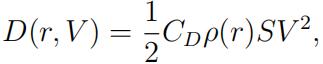
where
- CD = 0.3 is the drag coefficient;
- ρ(r) ≡ 1.225 kg/m3 is the air density (for simplicity we take it constant);
- S = 10.75 m2 is the reference area.
The gravitational acceleration is given by
where
- g0 = 9.8 m/s2 is the acceleration on Earth;
- R⊕ = 6,371 km is the Earth radius.
For the selected type of thruster, TM = 1,375.6 kN and ![]() [15 marks]
[15 marks]
Problem 2. Consider the plant Optimal Control代写
![]()
and the cost

a.Let α = 0 and x1(2) = 4. Express the optimal control in terms of the optimal costate.Write down the corresponding two-point boundary value problem. By solving this problem in Matlab (use bvp4c or bvp5c), find the optimal states and costates for β = 0, 0.1, 1, 10, 100. Plot your results in four subplots each showing one state/costate component for all β. For example, subplot(2,2,1) must show x1 for different β.
On the same axes but using dashed lines, plot the optimal states and costates for the case when α = 0 = β, x1(2) = 4, and x2(2) = 6. Add a legend, a title, and labels to each subplot.Explain what you observe and why.[25 marks] Optimal Control代写
b.Let α = 1 = β (free endpoint). Write down the boundary value problem to find the optimal control that guarantees
(x1(2) − 1)2+ (x2(2) − 1)2= 1.
Using Matlab, find and plot the optimal states, costates, and control. What are the values of x1(2) and x2(2)? Do they satisfy the terminal condition?[25 marks]