Case Western Reserve University Weatherhead School of Management
BAFI 435 – Empirical Finance Fall 2018
Assignment 3 (All Sessions) Due Wed, September 19th, 2018
This assignment will explore data extraction from WRDS. The objective is to prepare thedatasets that we will use in Module 4. Jumping ahead to Module 4, we will replicate a study reported in CLM about market reactions to earnings announcements. The main figure of the study is shown below:
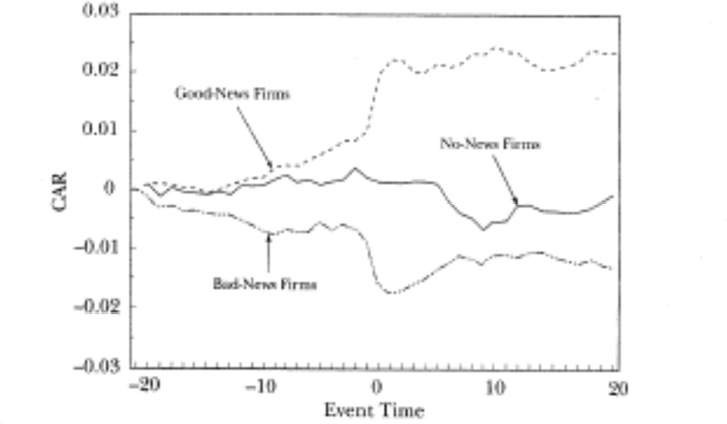
Figure 1. Market reactions to earnings announcements from Dow Jones’ firms, 1989-1993.
More specifically, we will look at market reactions to earnings announcements. Our sample will be quarterly earnings announcements for the 30 firms in the Dow Jones Index Average (DJIA), or simply Dow Jones index, between 1989 and 1993.
The assignment is an example of an empirical examination that depends on data collection from many different sources. Here, the following “files” will be involved:
- The list of firms that have been part of the Dow JonesIndex
- Data on earnings announcements for thosefirms
- Data on market expectations about earnings to bereleased
- Data on returns for thefirms
- Data on returns for the
Let’s proceed step by step.
- Icollected for you the components of the Dow Jones index between 1989 and The following table shows the data. For each component, I show the PERMNO, CUSIP, and the period the company was part of the index (that is between INIT_DATE and END_DATE). This table is saved as a simple text file DJIA_COMPONENTS_1989_1993.txt, available on Canvas.
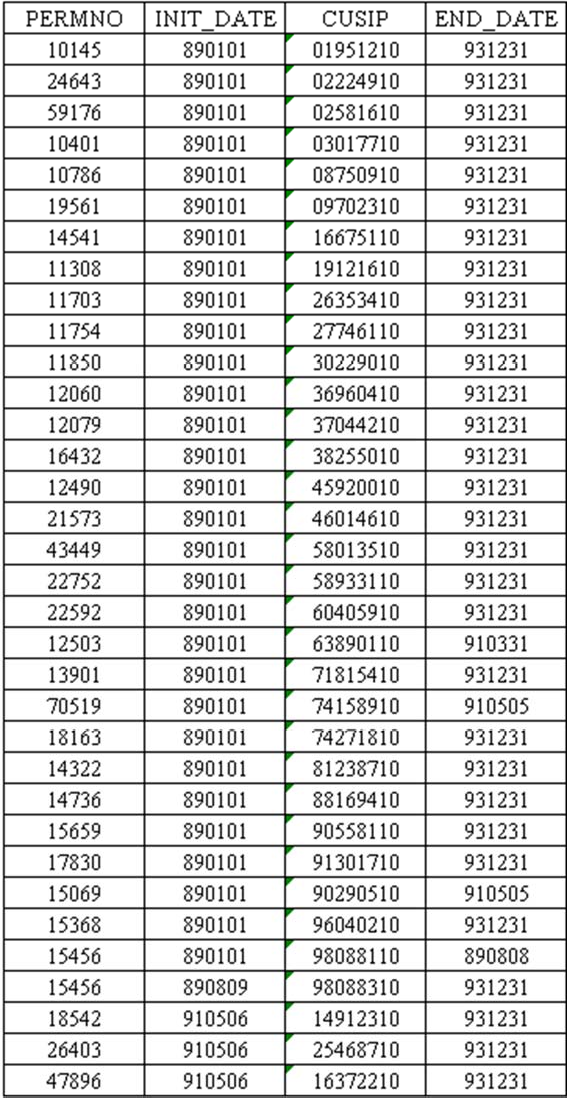
- Read this data into a SAS code. You can either read the file directly or copy and paste the contents of the file into your code and use the DATALINES statement. Force the CUSIP variable to be of the character datatype. Also, make sure you read the dates correctly by using the proper informat. After reading the dataset into your SAS code, print it to make sure the import worked.
- Hint: notice that there are more than 30 entries in the table above. This happens because companies go in and out of the DJIA index. See, for example, that PERMNO=15069 exited the index in May 5th, 1991.
- Now let’s work on the earnings data. Earnings data is collected by the IBES databasein WRDS, whose physical location is ‘/wrds/ibes/sasdata’. The first info we will collect refer to the quarterly earnings announcements. The IBES dataset ACTU_EPSUS contains such information. Create a library in your SAS code with a logical reference to the IBES directory and proceed with a PROC CONTENTS on the ACTU_EPSUS dataset. Take a look at the output. In particular, notice how many records the dataset
- You will see a bunch of variables. What you won’t see is a PERMNO variable. Instead, the identifiers for a company in IBES are CUSIP and OFTIC (the official ticker for the firm). Fortunately, you already have the CUSIP for the Dow Jones components, so you can search for a company’s earnings using its CUSIP.
- Start the data collection by obtaining data from ACTU_EPSUS for the sample of firms present in the Dow Jones index between 1989 and 1993. That is, combine the ACTU_EPSUS with your Dow Jones file based on the variable CUSIP, so that only observations from the ACTU_EPSUS that are also on the Dow Jones file are
- You should try a PROC SQL with a CREATE command to create such a table, similar to what we have done in Section 5 of Module 3. The PROC SQL should bring all variables from each dataset. The WHERE condition should match the CUSIP variable in each dataset. Look at the log file to note how many records were created in this new table.
- The final earnings table should have 600 observations (30 components of Dow Jones each quarter times 20 quarters). As of now, we have many more observations. This is because we did not put any other restriction on the data collection. For example, for PERMNO=10145 we are bringing many more earnings (annual, quarterly, before 1989, after1993, etc) than the 20 quarters we need from 1989 thru Our next step is to filter out the data we do not need. Here they are:
- The variable PENDS from ACTU_EPSUS indicates the quarter of the earnings observation. It is a variable stored as a date, more specifically, the last date of the calendarquarter to which that earnings data refers For example, earnings for the 2nd quarter of 2005 (which finishes in the end of June) will have PENDS=”30JUN2005”d. Thus, if I need the earnings data for the year 2005, I would use a restriction in my data collection as in “01JAN2005”d<=PENDS<=”31DEC2005”d. For our sample, Use the initial and end date from the Dow Jones table to restrict the quarters you are accessing; that is, you will need to write a filter such as INIT_DATE<=PENDS<=END_DATE.
- The variable PDICITY from ACTU_EPSUS indicates periodicity of the earnings data.Companies release both quarterly (PDICITY=”QTR”) and annual
- (PDICITY=”ANN”) earnings. Since our study uses quarterly earnings, you will need to restrict your data collection to observations with PDICITY=”QTR”.
- Earnings data includes information on various earnings measures, which are collected in different observations, as recorded in the variable MEASURE from ACTU_EPSUS: earnings per share (MEASURE=”EPS”), cash flows per share (MEASURE=”CFS”), etc. We will look at earnings per share only, thus restrict your data collection to observations withMEASURE=”EPS”.e a WHERE condition in a DATA step. For example, if the table from a) is named D, create a table E as
- data e;
set d
where <restrictions>;
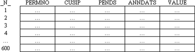
- Verify that your new table ends up with 600 observations. The additional variables you will need—besides the ones identifying the earnings (PERMNO, CUSIP, and PENDS)— are: the exact date of the announcement (ANNDATS from ACTU_EPSUS) and the actual value of the earnings that were announced (VALUE from ACTU_EPSUS). Thus, keep in your dataset only these variables. The dataset you want to create has the following format:
- IBES also records the output of sell-side analysts. In particular, IBES records detailed earnings forecasts by sell-side analysts. Besides detailed data, IBES records summary statisticson these forecasts, such as the mean forecast by these We will need these mean forecasts as a proxy for the market expectation on upcoming earnings.
- Let’s say that we wanted to know what was the market expectation, as of June 30, 2005, about the 2nd quarter of 2005’s earnings for IBM. This 2nd quarter’s earnings would be released sometime after June 30, 2005 (which is the end of the 2nd quarter). All we need to do is to look for the summary statistics on earnings forecasts for IBM around that specific date.
- Data on summary statistics on earnings forecasts is stored in the STATSUMU_EPSUS dataset of the IBES database. Please use the PROC CONTENTS on this dataset. An observation from this dataset is identified by the firm’s identifier (OFTIC, CUSIP), by the fiscal quarter it refers to (FPEDATS, equivalent to the PENDS variable in the ACTU_EPSUS dataset), by the type of the earnings number (FISCALP, equivalent to the PDICITY variable in the ACTU_EPSUS dataset), by the measure (MEASURE, as in the
- ACTU_EPSUS dataset), and by the date the summary statistics was computed (STATPERS variable).
- Thus, in our example above for IBM, I would look for the observations in the STATSUMU_EPSUS dataset that attend to the following clause:
- cusip=”45920010” and measure=”EPS” and fiscalp=”QTR” and fpedats=”30JUN2005”d and statpers<=”30JUN2005”d;
- Please try to collect the summary statistics data for IBM according to the above conditions. Please print these observations. How many such observations areavailable?
- You will notice that the clause above reads all summary statistics that were generated for that quarter for IBM, that is, potentially one generated in March 2005, another in April 2005, etc. An additional step would be to clean up the data to keep the one that is closest to June 30, 2005, that is, simply the latest such observation. In this case, it would be the observation with the STATPERS closest to June 30, 2005. What is the date (STATPERS) of this observation?
- Now, for the sample of earnings data you obtained in step 2, collect summary statistics onearnings forecasts that are available before the end of the fiscal Here you should use a PROC SQL so that you can match the summary stats dataset with the earnings dataset, based on CUSIP and the dates. For example, the search condition should include a restriction that the STATPERS in the summary stats dataset is smaller than or equal to the FPEDATS variable in the earnings dataset).
- The next step is to keep only the latest summary statistics for each quarter. The main variable you will need from the STATSUMU_EPSUS dataset is MEANEST (the average earnings forecast).
- Now, a hint on how you can “keep only the latest summary statistics for each quarter.” There are many ways to accomplish this, but here is one.
- Suppose you have a dataset D with all summary statistics for a quarter. Each observation is identified by the variables PERMNO, PENDS, and STATPERS. The idea is to use the NODUPKEYS clause in a PROC SORT; the clause keeps only one observation per set of variables identified in the BY clause. The code should be written as shown below:
- proc sort data=d;
by permno pends descending statpers;
proc sort data=d nodupkeys; by permno pends;
- This code sorts the D dataset by PERMNO, PENDS, then by the date the summary statistics was taken. The DESCENDING clause tells to sort by STATPERS in a descending fashion. The 2nd PROC SORT keeps only one observation per pair of PERMNO and PENDS, but since the dataset is already sorted by STATPERS (in an descending fashion), only the latest summary statistics is kept for each quarter.
- Let’slook inside the Read your datasets and extract the following information. For American Express (PERMNO=59176) and the quarter ending in September 30, 1991, what was the date of its earnings announcement? Which value for the earnings was announced at the time? What was the market expectation (mean estimate) for the upcoming earnings? When was that estimate produced? Was the newly announced earnings a positive or negative surprise with respect to what sell-side analysts were anticipating?
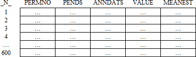
- Combine the data on earnings announcements and summary statistics in one single dataset. This final dataset should be named EARNINGS, and contain the following variables: PERMNO, PENDS, ANNDATS, VALUE, and MEANEST. Download this dataset to your SAS library in the Windows
- Make sure that this final dataset contains again 600 observations. That is, the format of your dataset should be:
- You will also need data on returns. For the sample described in step 1, collect the variables DATE and RET from the dataset DSF from the CRSP database (whose physical location is the directory‘/wrds/crsp/sasdata/a_stock’).
- Be careful here: the DSF dataset has return data on all public companies since 1926—you need returns only the sample of companies belonging to the DJIA over the period 1989- 1993. In other words, you should bring return data from DSF only for the firms that are also on the Dow Jones file you obtained in step 1). You can rely on a PROC SQL whose WHERE clause match PERMNOs from both files.
- Another restriction on which return data to bring is that returns should be collected in the period 01/01/1988 through 12/31/1994. (This is because we need data on early 1994 to analyze the earnings announcements from the last fiscal quarter of 1993.)
- Thus, create a dataset called RETURNS, with the following variables: PERMNO, DATE, and RET. The basic dataset should look like:
- Hint: since we have 33 companies and 7 years of daily returns, we should expect the number of observations N in the table above to be around 58,000 observations (each year has about 252 trading days, thus a first guess on the number of observations is 33*7*252=58,212). You can check using PROC CONTENTS if this guess is Ok.
- Download index returns (variable VWRETD) from the dataset DSIX (whose physical location is the directory ‘/wrds/crsp/sasdata/a_indexes’). Use the same period adopted in the previous step, 01/01/1988 through 12/31/1994. The final dataset should be named MARKET_RETURNS, and have the following variables: DATE (corresponding to the variable CALDT in the DSIX dataset) and VWRETD. The table islike:
- with a guess that N=7*252=1,764.
- Finally,some Your earnings dataset has the VALUE and MEANEST measures. For each observations in the earnings dataset, define a variable SURPRISE as VALUE minus MEANEST, then test the null hypothesis that analysts do a very good job of predicting earnings, that is, that surprise is on average zero,
- H0: E(SURPRISE) = 0
- Ha: E(SURPRISE) ≠ 0
- Compute the t statistic and the p-value, test the hypothesis (with a significance level of 5%), then define a 95% confidence interval for the SURPRISE measure. Discuss the results.
