EEE 6209
Advanced Signal Processing Coursework Report
Task 1: Signal analysis task
1) The number assigned to my signal is 76.
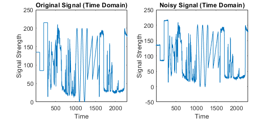
2) The original signal and noisy signal are plotted on Figure 1 using the plot function.
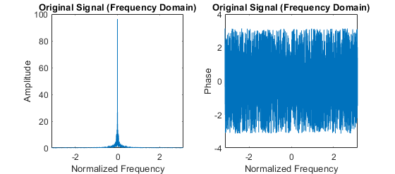
3) Apply FFT to the original signal and we obtain the FFT coefficients. The amplitude and phase are extracted from the FFT coefficients with abs and angle function in MATLAB respectively. Note that fftshift function is necessary to shift zero-frequency component to center of spectrum. The amplitude and phase of frequency components are plotted on Figure 2. Most of the original signal components are in the low-frequency part. The signal components with high frequency are extremely low.
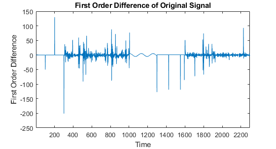
4) Time domain characteristics of the signal: As shown on Figure 1, the original signal consists of several typical waves: sinusoidal wave, triangular-wave and square-wave. Using moving difference filter , we can calculate the first order difference of the original signal, as shown on Figure 3.
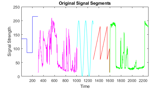
5) According to the shape of waveform and the edges in the first order difference, I divide the original signal into five segments manually. The starting and ending indices are 1 to 300, 301 to 1005, 1006 to 1298, 1299 to 1593 and 1594 to 2296. The segments are labeled with different colors on Figure 4.
6) Computation of Peak Signal to noise ratio (PSNR) for the noisy signal and its segments: We use the psnr function in MATLAB to calculate the PSNR value of noisy signal and signal segments. The results are as follows:
The PSNR value of the overall noisy signal is 46.6135dB.
The PSNR values of noisy signal segment 1,2,3,4,5 are 46.5662dB, 46.3791dB, 46.2641dB, 44.5220dB and 46.1651dB respectively.
7) Suggestion for noise removal strategies: The signal is of significant frequency domain characteristics that the signal components are mainly in the low-frequency. Therefore, it is straightforward to utilize the frequency domain characteristics to extract the original signal from the noisy signal.
Task 2: Fourier based denoising
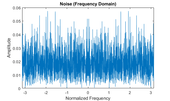
1) Noise plot: Apply FFT to the noise and the FFT coefficients are obtained. The amplitude values of FFT coefficients are calculated with abs function in MATLAB. The fftshift function in MATLAB is used to shift zero-frequency component to center of spectrum. The amplitude of FFT coefficients of the noise are shown on Figure 5. We can see that the amplitudes are larger than zero, which means that the noise spreads in all frequencies.
2) After applying FFT to the original signal, we find that a small part of FFT coefficients have a large percent of energy of the overall signal. Because the amplitudes of noise FFT coefficients are smaller than the amplitudes of signal FFT coefficients, we can remove the FFT coefficients with small amplitudes and then reconstruct the original signal from the remaining FFT coefficients.
The pseudo code of FFT based denoising is as follows:
Algorithm 1: FFT based denoising
Input: Signal x, number of remained FFT coefficients n
Output: Denoised signal y
- X FFT(x)
- Index Sort(X, ‘descend’)
- fori = 1; i <= n; i++
- Y(Index(i)) = X(Index(i))
- end
- fori = n+1; i <= length(X); i++
- Y(Index(i)) = 0
- end
y IFFT(Y)
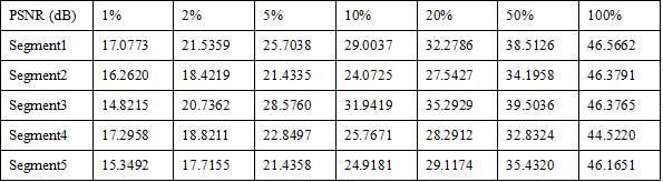
The PSNR values of recovered signal segments with different number of selected FFT coefficients are shown on Table 1. As we can see, for each signal segment, the PSNR value increases with more selected FFT coefficients.
When 100% of FFT coefficients are selected for signal recovery, the PSNR of recovered signal segment equals to the PSNR value of original signal segment.
Figure 6. Recovered signal segments using FFT
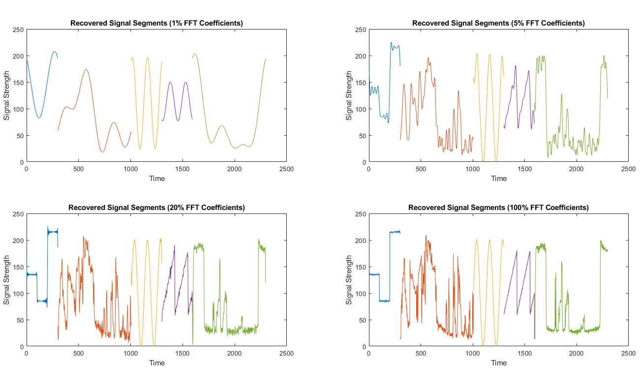
- If we fix the ratio is 1%/5%/20%/100%, which means 1%/5%/20%/100% of FFT coefficients with the largest amplitudes are kept for signal recovery respectively, the recovered signal segments are shown on Figure 6.
- As we can see, if a small part (e.g., 1%) of FFT coefficients are used for signal recovery, the resulting recovered signal segments only consist of several sinusoidal waves. The shape of the recovered signal is far away from the original signal, which means that a small part of FFT coefficients are not enough for signal recovery.
- When the kept FFT coefficients becomes more and more, the recovered signals are more and more similar to the original signal and the PSNR values increases.
- It can be observed that the PSNR value is not very high, the reason lies in two folds. On one hand, the FFT coefficients with larger amplitudes that we choose to recover original signal segments also contain the noise.
- By choosing a larger percent of FFT coefficients, more noise is attained in the recovered signal. On the other hand, the dropped FFT coefficients contain the original signal, if a smaller percent of FFT coefficients are attained, a part of original signal is removed with noise at the same time.
- To summarize, the frequencies of original signal and noise are overlapped. Therefore, it is hard to completely remove the noise from the signal based on FFT.
Task 3: DCT based denoising
Similar to FFT based denoising, when we apply DCT to the signal, we also find that a few DCT coefficients of the signal have a large percent of signal energy. Therefore, we keep the DCT coefficients with large amplitudes and remove DCT coefficients with small amplitudes. The original signal is recovered by applying IDCT to the remaining DCT coefficients.
The pseudo code of DCT based denoising is as follows:
Algorithm 2: DCT based denoising
Input: Signal x, number of remained DCT coefficients n
Output: Denoised signal y
- X DCT(x)
- Index Sort(X, ‘descend’)
- fori = 1; i <= n; i++
- Y(Index(i)) = X(Index(i))
- end
- fori = n+1; i <= length(X); i++
- Y(Index(i)) = 0
- end
- y IDCT(Y)
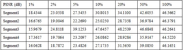
The PSNR values of recovered signal segments with different number of selected DCT coefficients are shown on Table 2. For each signal segment, the N parameter of DCT equals to the length of the signal segment. Therefore, the number of N-point DCT coefficients equals to the number of FFT coefficients. Similar to the results of Table 1, for each signal segment, the PSNR value increases with more selected DCT coefficients. When 100% of DCT coefficients are selected for signal recovery, the PSNR of recovered signal segment equals to the PSNR value of noisy signal segment.
It can be also noticed that in the same row and same location of Table 1 and Table 2, the PSNR value in Table 2 is always larger than the PSNR value in Table 1, which means with the same number of coefficients, the DCT based signal recovery outperforms FFT based signal recovery. We can conclude that DCT can make the signal energy more compact than FFT.
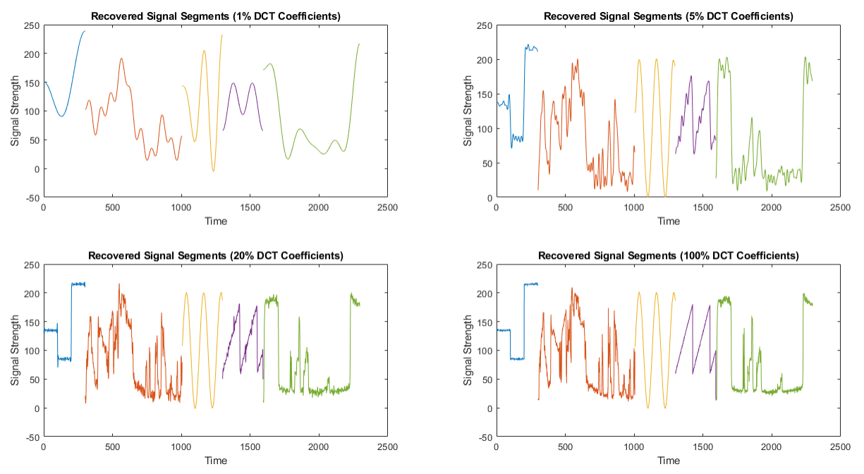
We also select 1%/5%/20%/100% of DCT coefficients with the largest amplitudes for signal recovery respectively, and the results are shown on Figure 7. Similar to FFT based signal recovery, the quality of DCT based denoising is also better with more DCT coefficients, as demonstrated in both the PSNR values in Table 2 and the curves in Figure 7.
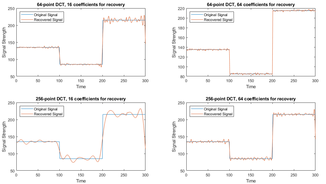
Moreover, we repeat the experiment under different N parameters. Take signal segment 1 as an example, we apply 64/256-point DCT respectively. Under different number of DCT coefficients, we repeat the above experiment. As shown on Table 3, with more points, DCT based signal recovery achieves higher PSNR with the same percent of DCT coefficients. However, if we fix the absolute number of selected DCT coefficients, the results will be different. With the same number of DCT coefficients, 64-point DCT outperforms 256-point DCT. This is also demonstrated on Figure 8. The signal recovered from 16 coefficients of 64-point DCT is more similar to the original signal than that recovered from 16 coefficients of 256-point DCT.
| PSNR (dB) | 1% | 2% | 5% | 10% | 20% | 50% | 100% |
| 64-point DCT | 15.9215 | 15.9215 | 20.9401 | 24.5999 | 28.8168 | 33.9461 | 46.5662 |
| 256-point DCT | 16.1275 | 19.1551 | 23.2324 | 26.1174 | 29.5954 | 36.0217 | 46.5662 |
Table 3. PSNR values of recovered signal segments using different point DCT
| PSNR (dB) | 4 | 8 | 16 | 32 | 64 | 128 | 256 |
| 64-point DCT | 22.318 | 25.4255 | 30.2428 | 33.9461 | 46.5662 | \ | \ |
| 256-point DCT | 18.8217 | 20.8759 | 23.8518 | 27.151 | 30.7719 | 36.0217 | 46.5662 |
Table 4. PSNR values of recovered signal segments using different point DCT
Overall Comparison and Discussion
From the above experiment, I conclude FFT and DCT can both be applied for signal denoising. By applying FFT/DCT to the signal, we can get a series of FFT/DCT coefficients. The coefficients with large amplitudes indicate the signals, while those with low amplitudes are actually brought by the noise. Therefore, the original signal can be recovered by removing the coefficients with low amplitudes and applying IFFT/IDCT.
However, FFT and DCT poses different characteristics.
On one hand, DCT is better in terms of energy compaction, which means the majority of energy comes from a few DCT coefficients. To achieve the same signal recovery quality, more FFT coefficients are needed than DCT coefficients.
On the other hand, the DCT parameter N can be adjusted. Experimental results show that it is not necessary to apply a large number of points DCT and a small number of points DCT can achieve comparable signal recovery quality if we select suitable number of DCT coefficients. It inspires us that DCT can effectively compress various signals, including audio and image signals.
获取关于“信号处理代写 EEE 6209 Advanced Signal Processing”的需求页面!
如果使用请联系作者,否者请侵权!
