
Economics 4261 Introduction to Econometrics
ECON 4261: Problem Set 4
ECON 4261代写 Selection Bias.We want to study the effffect of health insurance on health. For the moment, imagine that we only have data for ···
Exercise 1 ECON 4261代写
Selection Bias.
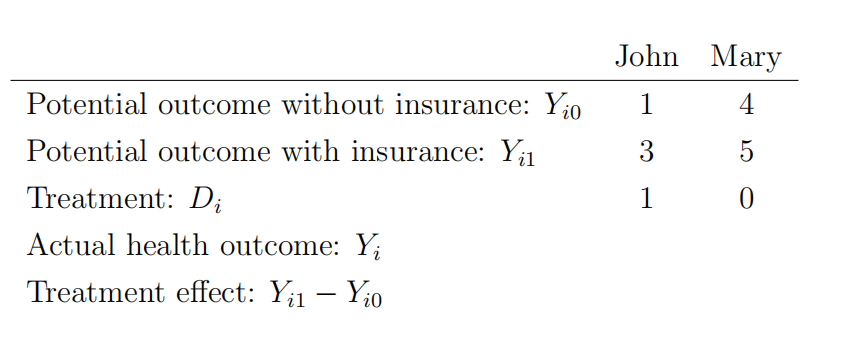
We want to study the effffect of health insurance on health. For the moment, imagine that we only have data for two individuals, John and Mary. Health is measured from 1 to 5. Yᵢ is the actual outcome for individual i, Dᵢ is the selection variable (0=no insurance, 1=insurance) and Yᵢ₁, Yᵢ₀ are the potential outcomes for the same individual i with and without insurance.
a Complete the values in the table for the actual health outcome, Yᵢ , and the treatment effffect, Yᵢ₁ − Yᵢ₀.
b Imagine that we just compare the actual outcome for John and Mary. What do you fifind? Can we interpret the difffference as the causal effffect of having an insurance on health? Explain.
Imagine we now have access to data for a lot of individuals with and without insurance.
c Comparing their outcomes we can compute:
E[Yᵢ₁|Dᵢ = 1] − E[Yᵢ₀|Dᵢ = 0]
Show mathematically that this number can be expressed as the sum of the average causal effffect and a selection bias term.
d Describe a situation where the selection bias is zero and we can interpret directly the difffference between observed outcomes as the causal effffect of having a health insurance on health.
Exercise 2 ECON 4261代写
Estimation of a Wage Equation using IV.
This exercise illustrates the use of instrumental variables to isolate the ef-fect of education on the wage rate from that of ability. We are going to follow Griliches (1976), a classic study of the determinant of wages. The fifile griliches.xls¹ contains a sample of 758 young men. We are going to use the following variables: s, expr, and tenure (years of schooling, experience, and job tenure, respectively); rns, an indicator for residency in the South; smsa, an indicator for urban versus rural² ; and year (we need to control for year effffects). Also we will need: iq, the worker’s IQ score, med, the mother’s level of education; kww, the score on another standardized test; age, the worker’s age; and mrt, an indicator of marital status (1 if married).
1
Calculate the descriptive statistics (mean and standard deviation) of all these variables and the correlation between s and iq. Report the results in a table. Hint: Use the command summarize and correlate in STATA.
2 ECON 4261代写
Generate eight year dummies (notice that there is no observation for 1972) We want to include year dummies in our model to control for year effffects³.
Hint: To generate the regressors year66, for example, you can use the following code in Stata:
generate year66 = 0
replace year66 = 1 if year == 66.
It is a good idea to browse your data (‘Data’, ‘Data Editor’, ‘Data Editor (Browse)’) to check that you generated the variable you intended to create.
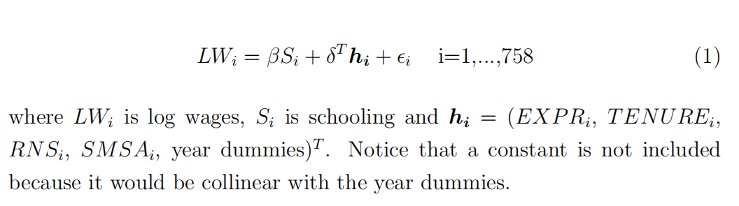
Consider the following regression equation for the wage equation (in matrix
form):
3
Estimate the regression equation (1) using OLS and report the coeffiffiffi-cient for schooling (which is our variable of interest), the standard error and R² . Do you think that β is biased in this model? Explain your answer and argue brieflfly whether OLS over- or under-estimates the effffect of schooling on wages. Hint: Should ability belong to the true model? If so, use the correlation in part 1 to argue the sign of the bias?
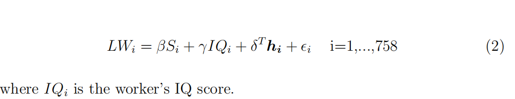
In the previous part, we learnt that there may be a problem with our model. We are missing an important variable: ability. However, our dataset includes a variable that we can use as a proxy for ability: iq. Therefore, consider the following regression equation:
4
Assume that IQ is a measure of ability which is exogenous. Estimate the model (2) using OLS. Report the coeffiffifficients for schooling and IQ, the standard errors and R² . Compare the coeffiffifficient for the effffect of schooling with the one obtain in (1). Why is it lower now?
Now, let’s assume that IQ score is endogenous. Endogeneity can affffect the estimation of the rest of the coeffiffifficients. In particular, it can affffect the effffect of schooling on wages. Therefore we want to use Instrumental Variables to solve this problem.
5 ECON 4261代写
We have 4 possible candidates to be used as instruments of IQ: med, the mother’s level of education; kww, the score on another standardized test; age, the worker’s age; and mrt, an indicator of marital status. Compute the fifirst stage for these instruments (and report your results) and argue whether they are good instruments. Do they have a signifificant effffect on IQ? Hint: Run a regression of IQ (the endogenous variables) on all the exogenous variables of our model (2) and the four instruments. We want to check whether our instruments are correlated with our endogenous variable so we can argue whether they are good instruments.
From the last question we know that we have available 4 difffferent instruments and we just have one endogenous variable, IQ. The model is over identifified. As we learnt in class, we can apply 2SLS (also known as Generalized IV).
6 Estimate (2) using 2SLS. Use all four instruments. Report the coef-fificients for schooling and IQ, the standard errors and R² . Do your results change with respect to question 3 and 4? Explain. Hint: Use the command ivreg₄ in STATA.
Exercise 3 ECON 4261代写
The Wald Estimator and the effffect of compulsory schooling on wages.
Consider the simple regression model:
y = β₀ + β₁x + ∈
and let x be an endogenous variable and z be a binary instrumental variable for x. Assume that we observe a random sample {(yi , xi , zi)Ni=1}. Further assume that for N1 observations zi = 1 and for N0 observations zi = 0 such that N = N₁ + N₀.
1
Construct the matrix X (a N × 2 matrix including the variables in the model) and W (a N ×2 matrix with all the weakly exogenous variables of the model).
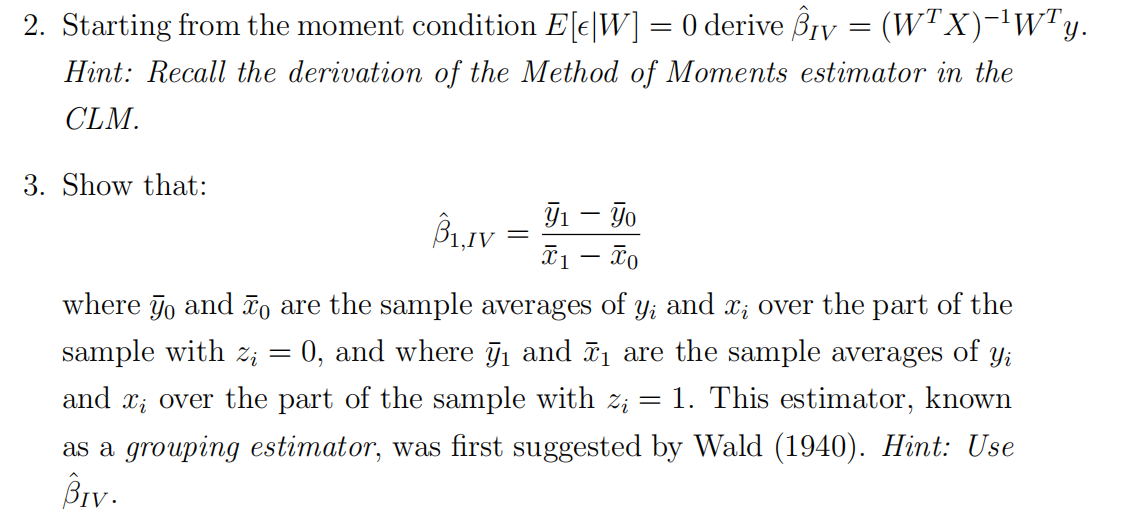
Angrist and Krueger (1991)⁵ estimate the effffect of compulsory schooling on wages. They use the same model that we have (plus a set of extra control variables that we ignore) where: y is wages, x is years of schooling and z is quarter of birth (0=Jan-Sept, 1=Sept-Dec). In order to construct their instrument they use two institutional features of the US educational system:
– A student can “only” enter school (fifirst grade) if she will be 6 years old by Jan. 1 of the academic year in which she starts school. ECON 4261代写
– A student must remain in school until age 16.
This implies that people with z = 1 are forced to complete more years of schooling before they can drop out. For example, children born in 2000 can drop out on their birthday in 2016. Those with z = 0 will be in ninth grade; those with z = 1 will be in tenth grade.
4
Argue why the quarter of birth is a valid instrument.
5
What condition should it satisfy to be a good instrument ? Do you think it is satisfified in this case? Explain.
6
What is the interpretation of the Wald estimator (computed in part 3.) for this particular example?

其他代写:homework代写 Exercise代写 essay代写 英国代写 作业代写 CS代写 Data Analysis代写 data代写 澳大利亚代写 app代写 algorithm代写 作业加急 加拿大代写 北美代写 北美作业代写 assignment代写 analysis代写 code代写 assembly代写
合作平台:essay代写 论文代写 写手招聘 英国留学生代写
