Statistics作业代做 STA255H1代写 Statistical Theory代写

STA255H1: Statistical Theory

Assignment

Winter 2020

Submission deadline: Mar 30, 11.59pm (Late submissions will not be accepted)

Statistics作业代做 Using the table of proportions or otherwise, calculate the mean of these 125 numbers (valuesunder X bar) and compare

Instructions on completing the assignment

The numerical calculations involved in this assignment are simple and you are already familiar with them (hopefully). The goal of this work is to help you “see” some of the theorems and concepts we have learned or used in this course using empirical data. Calculations are mostly repetitive in nature! I suggest using R (or any other programming language that you are comfortable with). If you don’t feel comfortable with R, for question 1 and 2, you can use microsoft excel.

Instructions on creating documents for submission

Please create 3 separate pdfs (one for eachquestion).
If you are familiar with R-markdown please use it. If you are not familiar with R-markdown, you can write your answers using microsoft word and in the end save it as pdfs. Pdf is the only acceptable format offtles.
We will use crowdmark for submission and grading. You will have to upload three separate documents as your answers to three separate questions. Crowdmark links to upload your documents will be emailed to you later this week.

Academic Integrity

You are allowed work in pairs. If you need clarification on any of these questions, you are allowed to ask questions on Piazza. Don’t ask for solutions to anyone. Do not share your codes or answers on any platform with anyone other than your assignment partner.

Question 1 [10 points].

Suppose you have a population of size 5 [i.e. N=5]. You measure some quantity (X) and the corresponding numbers are:

21, 22, 23, 24, 25

a) Calculate the population mean (µ)

b) Calculate the population variance (σ2 ) using the formula

c.Imagine you are taking samples (of size n = 3) from this population with replacement.

Write down every possible way that you could have a sample of size 3 with replacement from this population. (hint: there will 5*5*5 = 125 possible combinations)

Help: if you are struggling with figuring out the combinations try this code in R: expand.grid( c(21:25), c(21:25), c(21:25) )

d)For each of these samples of size 3, calculate the sample mean and record it (either as a new object in R or as a new column if you are using excel). Lets call this new column X bar. So you should have 125 values in this column.

e)You should have noticed that the values in the X bar column are repetitive.For example, 21.3333333 will show up 3 times.

Construct a frequency table based on the column X bar. [i.e. write down which values showed up how many times]. Now using the frequencies (also known as counts) calculate proportion of each of those repeated values. [For example: proportion of 21.3333333 will be 3/125]

f)Plot these proportions against the values and connect the points using a non-linear line. Doesthe shape of this plot look like any known distribution? Name the distribution.

g)Using the table of proportions or otherwise, calculate the mean of these 125 numbers (valuesunder X bar) and compare it to your answer of 1(a).

h)Usingthe table of proportions or otherwise, calculate the variance of these 125 Use the population variance formula (i.e. divide by 125 not 124). What is the relationship of this answer to your answer of 1(b)?

i)Which theorem did you demonstrate empirically in part f, g andh?

(No output needed for part(c and d) of this question)

Question 2 [10 points].

This question continues from question 1(c). For each of these sample of size 3, calculate the sample variance using the following two formulas

Assume the population variance, σ² = 2.

(you should get 125 different values of S² and and 125 different values of σˆ²)

a.By calculating (numerically using the 125 different values) Bias[S²] and Bias[σˆ²] check the unbiasedness of these two estimators.

b.By calculating all three components separately check the followingidentity

M SE[σˆ²] = var[σˆ²] + (Bias[σˆ²])²

Question 3 [10 points].

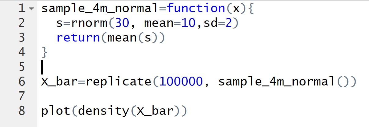
In week 6, we demonstrated an R code that replicates the sample distribution of X¯ . Here is the code that was used in the lecture.

Simply change the distribution and number of samples on line 2 of this code to do this question. Search online for this keywords : ”runif” and ”rchisq”.

Produce the density of

a)whenn = 2, X ∼ U nif [0, 1]

b)whenn = 5, X ∼ U nif [0, 1]

c)when n = 5, X ∼χ²

d)when n = 30, X ∼χ²

e)when n = 5, X ∼χ²

(Ans to part(a) to Pat(e) are 5 different graphs)

f)CLTsays for large n, X¯ converges(in distribution) to a Normal

By comparing your graphs from parts (a) to (e), can you comment on how large n has to be in order for X¯ to converge to a Normal distribution.

g)A quick way to plot any distribution in R is to draw a large sample from a distribution and plot its For example ”plot(density(rnorm(100000,mean=10,sd=2)))” will produce a N(10,4)curve.

Plot three separate density curves for U nif [0, 1], . Looking at the skewness of these three curves, what comments can you make on the question asked in part(g)?

合作平台：essay代写论文代写写手招聘英国留学生代写