Project Grading Rubric
2018-11-26
Data source and describe
The data came from kaggle, an algorithm competition website.The specific website is: https://www.kaggle.com/loganalive/echocardiogram-uci .This dataset consists of 132 instances of patients for 12 variables describing the patient’s heart attack and condition.I selected 8 important variables as the data for this analysis, which are specifically described as follows:
1 survival: The number of months a person survived from heart disease was recorded. 2 still-alive: s the patient still alive? 0 means dead , 1 means still alive.
- age:age in years when heart attack
- pericardial-e”usion:Pericardial e”usion is fluid around the 0=no fluid, 1=fluid.
- fractional-shortening:a measure of contracility around the heart ,lower numbers are increasingly
- epss: E-point septal separation, another measure of contractility. Larger numbers are increasingly
- lvdd:left ventricular end-diastolic Large hearts tend to be sick hearts. 8 wall-motion-index: a measure of how the segments of the left ventricle are movin
Question
All the patients had experienced heart attacks in the past.Some are still alive, some are dead for a short time.I want to know which variables have an important e”ect on this di”erence in outcome.Pericardial e”usion is a response to damage to the parietal pericardium and can cause other complications.Whether pericardial e”usion significantly a”ects the time of death in patients with heart disease.
#Load the required packages and data library(ggplot2)

library(survival) library("survminer")

echocardiogram<-read.csv(file="echocardiogram.csv")
#Data cleaning and variable selection echocardiogram<-na.omit(echocardiogram[,c(1:7,9)])
Variable analysis
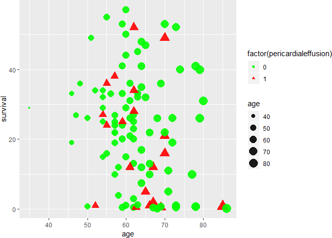
As can be seen from the figure below, there is no significant di”erence in survival time between patients with pericardial e”usion and those without e”usion. The age of patients with pericardial e”usion is more concentrated, between 50 and 70 years old.
ggplot(echocardiogram, aes( x = age, y = survival, color = factor(pericardialeffusion), size = age, shape = factor(pericardialeffusion)))+

geom_point(alpha = 0.9)+ scale_color_manual(values=c('green','red'))
ggplot(data=echocardiogram, aes(x=factor(alive),y=survival))+geom_boxplot(aes(fill=factor(pericard
The survival curve of patients with heart disease was drawn only considering whether there was pericardial e”usion or not. As can be seen from the picture, the survival rate of heart patients with pericardial e”usion is lower than that of heart patients with pericardial e”usion over time.
fit1 <- survfit(Surv(survival,alive)~factor(pericardialeffusion),data=echocardiogram) plot(fit1,mark=19,lwd=2,col=c(4,2), ylab="Survival Proportion", xlab="Months") legend(10,0.4,c("no fluid","fluid"),fill=c(4,2))

Cox PH regression
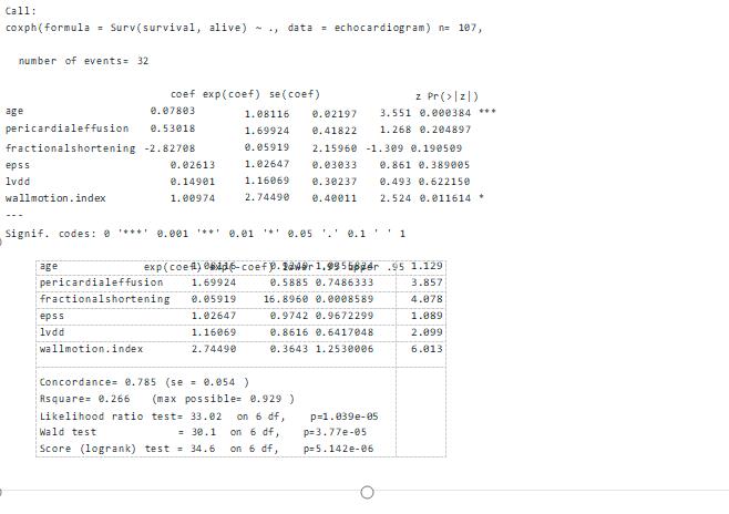
Now we’re going to describe how some of these factors come together to influence survival.To answer this question, we will perform a multivariate Cox regression analysis. In multivariate Cox analysis, age and wallmotion index were significantly correlated (p<0.05).Pericardial e”usion was not significant (P = 0.20, which was larger than 0.05).Similarly, fractional shortening, epss, and LVDD have P values greater than 0.05, indicating that they contributed less to the di”erence in survival time.The age p value was 0.000384, the risk ratio HR = exp (coef) =1.08116, and the 95% confidence interval (1.0355824, 1.129), indicating a strong relationship between the age of patients and the risk of death.The pericardial e”usion p value was 0.204897, the risk ratio HR = exp (coef) =1.6994, and the 95% confidence interval was (0.7486333, 3.857), indicating that there was also a strong relationship between patient pericardial e”usion and the reduced risk of death, but the fluctuation range was large.The risk ratio of covariates can be explained as the multiplier e”ect on risk.For example, fluid (pericardial e”usion= 1) that remains the same for other covariables increases the risk to 1.6994 times, that is, a 70 percent increase.We conclude that fluid patients are more likely to die.
fit2<- coxph(Surv(survival,alive)~.,data=echocardiogram) summary(fit2)
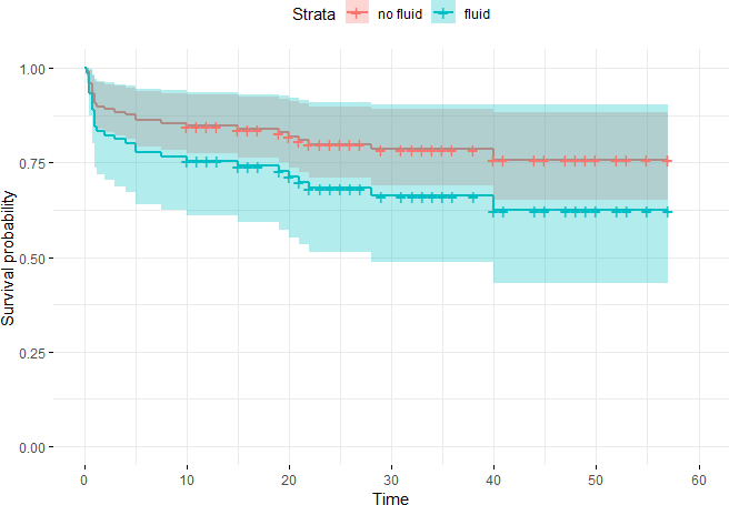
As can be seen from the figure below, the survival curve of heart patients with pericardial e”usion is lower than that of heart patients without pericardial e”usion, which indicates that heart patients with pericardial e”usion are more likely to die. The confidence interval of pericardial e”usion survival curve is very large, covering the confidence interval of non-e”usion survival curve, which indicates that the reliability of the results has some problems.
df<-with(echocardiogram,data.frame(pericardialeffusion=c(0,1),age=rep(mean(age),2), fractionalshortening=rep(mean(fractionalshortening,na.rm=TRUE),2), epss=rep(mean(epss,na.rm=TRUE),2),

lvdd=rep(mean(lvdd,na.rm=TRUE),2), wallmotion.index=rep(mean(wallmotion.index,na.rm=TRUE),2)))

curvesfit<-survfit(fit2,newdata=df) ggsurvplot(curvesfit,data=df,conf.int=TRUE,legend.labs=c("no fluid","fluid"),

ggtheme=theme_minimal())
Model Fitting, using AIC to pick the right set of covariates
We use stepwise regression to optimize our model variables. After stepwise regression, we retained three variables: epss, wallmotion index and age.Compared with the unoptimized model, the P values of Likelihood ratio test, Wald test and Score (logrank) test are all reduced by an order of magnitude. After optimization, the P values of the three overall tests of the model are far less than 0.05, which indicates that the model is significant on the whole. The P values of all three variables were less than 0.05, indicating that three variables were significantly correlated with survival time.
fit3<-step(fit2)
Start: AIC=261.56

Surv(survival, alive) ~ age + pericardialeffusion + fractionalshortening + epss + lvdd + wallmotion.index


Df AIC

- lvdd 1 259.81

- epss 1 260.29
-
pericardialeffusion 106
-
fractionalshortening 137
<none> 261.56
-
index 1265.36
- age 1 271.71


Step: AIC=259.81

Surv(survival, alive) ~ age + pericardialeffusion + fractionalshortening + epss + wallmotion.index


Df AIC
-
pericardialeffusion 152
<none> 259.81
-
fractionalshortening 194
- epss 1 259.98
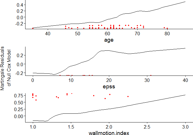
In general, we assume a linear relationship between covariates and-log(s(t)). Nonlinear diagnosis of model covariates can be achieved by drawing Martingale residual diagram. Nonlinear diagnosis is generally aimed at continuous variables in the model. As shown in the figure below, although the variables have a local non-linear trend, the overall trend is linear.
gcoxfunctional(fit3,data = echocardiogram)
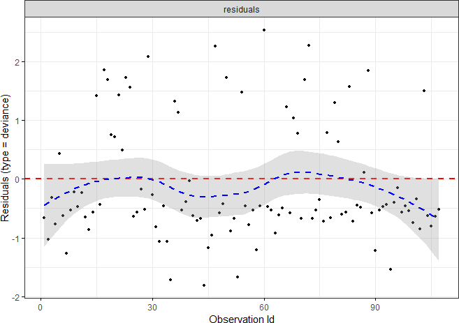
The residual values are uniformly distributed around 0, indicating that the model conditions are satisfied.
ggcoxdiagnostics(fit3,type = "deviance",

linear.predictions = FALSE,ggtheme = theme_bw())
ggcoxdiagnostics(fit3,type = "dfbeta",

linear.predictions = FALSE,ggtheme = theme_bw())
Extension
Heart disease patients are always concerned about how long they can survive. It is di cult to predict the survival time of patients accurately. We can reduce the di culty of judging whether a patient can survive for more than a year. According to survival and survival variables, we can judge whether patients survive for more than one year. I can derive a new binary variable, aliveat1. 0 refers to patients who died within one year or followed up for less than one year. 1 represents that the patient has survived for more than one year. We can predict whether a patient will survive for more than a year based on the variables available. Decision trees or random forests are my priority models. However, there may still be a problem. There are only 122 samples in the data set, which is a big challenge to the accuracy of the model.
