最近某项目要搞数据挖掘,需要对数据举办可视化显示,原本我是规划直接用Excel 算了,规划,用了一段时间,发明有些数据图用excel贫苦得要命,然后,上网找了一下,本来,有在这方面也有一门专门的语言—-R语言,我发明,用它绘制数据图十分强大,就规划花几天,就进修如何用R语言绘制数据图
散布图(scatter plots)
需要把握的呼吁:
plot()
xyplot()
qplot()
text()
smoothScatter()
matrix()
jitter()
rbinom()
rnorm()
lines()
lowess()
nls()
用的的包:
ggplot2
lattice
scattersplot3d
辅佐用法:
呼吁行内里直接打
?你要查的呼吁即可
基本用法:
?
1 |
plot(cars$dist~cars$speed)
|
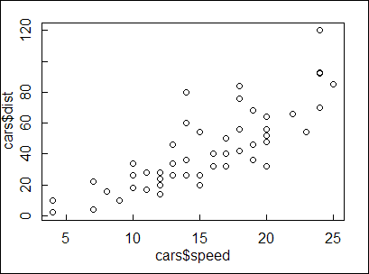
更多用法在R节制台中打上
?
你就清楚用法了
xyplot
数据汇总要领
?
1 |
xyplot(Sepal.Length~Sepal.Width,data=iris,groups=Species,auto.key=list(corner=c(1,1)))
|
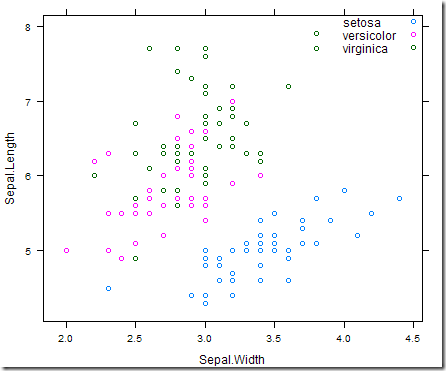
格栅
qplot()
?
1 |
qplot(Sepal.Length,Sepal.Width,data=iris,col=as.factor(Species),size=as.factor(Species),shape=as.factor(Species))
|
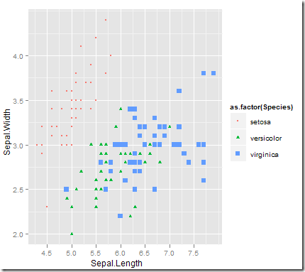
标识点
?
1
2 |
plot(mpg~disp,data=mtcars)
text(160,21,“Mazdz RX4”)
|
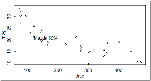
发抖(jitter)
?
1
2
3 |
x <- rbinom(1000, 10, 0.25)
y <- rbinom(1000, 10, 0.25)
plot(x, y)
|
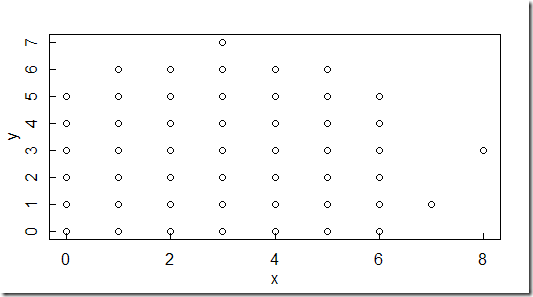
发抖后
?
1 |
plot(jitter(x),jitter(y))
|
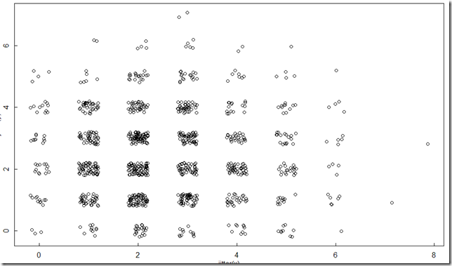
x所有点都可以显示出来
直线模式:
?
1
2
3 |
plot(mtcars$mpg~mtcars$disp)
lmfit <- lm(mtcars$mpg~mtcars$disp)
abline(lmfit)
|
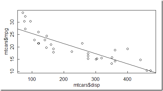
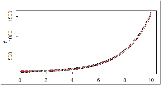
非线性模式的曲线:
?
1
2
3
4
5 |
x <- -(1:100)/10
y <- 100+10*exp(x/2)+rnorm(x)/10
nlmod <- nls(y~Const+A*exp(B*x),trace=TRUE)
plot(x,y)
lines(x,predict(nlmod),col=“red”)
|
非参数值的曲线(英文是non-parametric,我也搞不清楚这样相识对差池)
?
1
2
3 |
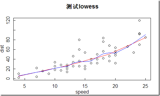
plot(cars, main=“测试lowess”)
lines(lowess(cars), col=“red”)
lines(lowess(cars, f=0.3), col=“blue”)
|
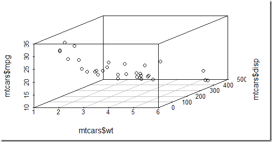
建造3D视图
需要利用 scattersplot3d 包
?
1 |
scatterplot(mtcars$wt, mtcars$disp, mtcars$mpg)
|
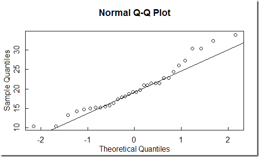
QQ图(研究正态漫衍的一种图…)
?
1
2 |
qqnorm(mtcars$mpg)
qqline(mtcars$mpg)
|
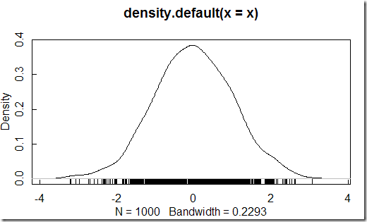
在坐标轴上显示数据密度
?
1
2
3 |
x <- rnorm(1000)
plot(density(x))
rug(x)
|
大数据的滑腻分手图显示
?
1
2
3
4 |
n <- 1000000
x <- matrix(rnorm(n), ncol=2)
y <- matrix(rnorm(n,mean=3,sd=1.5), ncol=2)
smoothScatter(x,y)
|
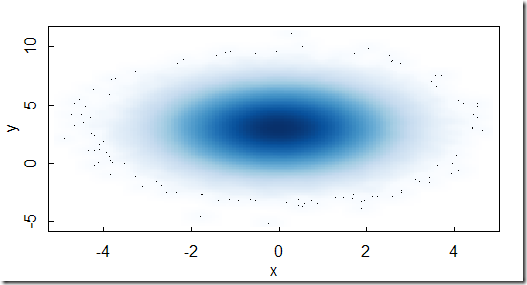
这么看正态漫衍图挺带感的