Forecasting代写 Assignment代写 Model Selection代写

MgtF 405: Forecasting

Forecasting代写 This assignment uses the file Goyal_Welch_data2016.xlsx in the Assignment 2 folder on Triton ED. The data is downloaded

Assignment 2 (due on January 25, 2019)

Part I. Model Selection Forecasting代写

This assignment uses the file Goyal_Welch_data 2016.xlsx in the Assignment 2 folder on Triton ED. The data is downloaded from Amit Goyal’s web site and is an extended version of the data used by Goyal and Welch (Review of Financial Studies, 2008). It contains monthly information on US stock returns as well as on a range of predictor variables proposed in the literature. We have also provided matlab and R codes for you to use in the analysis (available in the Assignment 2 folder).

You are asked to estimate forecasting models and simulate their performance out-of-sample. To do so, use data from 1927m1 to 1969m12 to estimate each forecasting model, then generate a return forecast for 1970m1. Then add the monthly data for 1970 to the estimation model and produce a forecast for 1970m2. Repeat this process until the end of the sample in 2016m12. This is called back testing or simulated out-of-sample forecasting. Forecasting代写

Each forecasting model has the excess stock return as the dependent variable.

The excess stock return is listed in column E (as a rate of return per month). As predictors you can choose from a list of 10 variables: the dividend-price ratio D/P (col F), earnings-price ratio E/P (col G), book-to-market ratio b/m (col H), T-bill rate tbl (col I), default-spread def_spread (col J), long-term yield lty (col K), net equity issues ntis (col L), inflation rate infl (col M), long-term returns ltr (col N), and stock variance svar (col O). The definition of these variables is explained in Goyal and Welch (2008).

Estimate linear regression models of the form (where y_t+1 = excess return_t+1 from col. E)

(1)

Make sure to use one-month lagged values of the predictors. Univariate models have only a single predictor x₁. Multivariate models have two or more predictors x₁, x₂,…. All models include an intercept term.

1.At each point in time where you are generating a forecastForecasting代写

(1969m12, 1970m1, .., 2016m11) find a way to select a preferred forecasting model. You can do this by using stepwise selection methods (general to specific or specific to general) or you can do this by conducting an exhaustive model selection search over all 2¹¹possible regression models, selecting the model by AIC or SIC. Or, you can use another method such as LASSO. Plot the forecasts against the actual values and report the root mean squared forecast error associated with the forecasts.

Sol: The exhaustive model selection search over all 2¹¹ possible regression models is conducted. The model is selected by SIC.

The plot of forecasts against the actual values is shown in below figure.

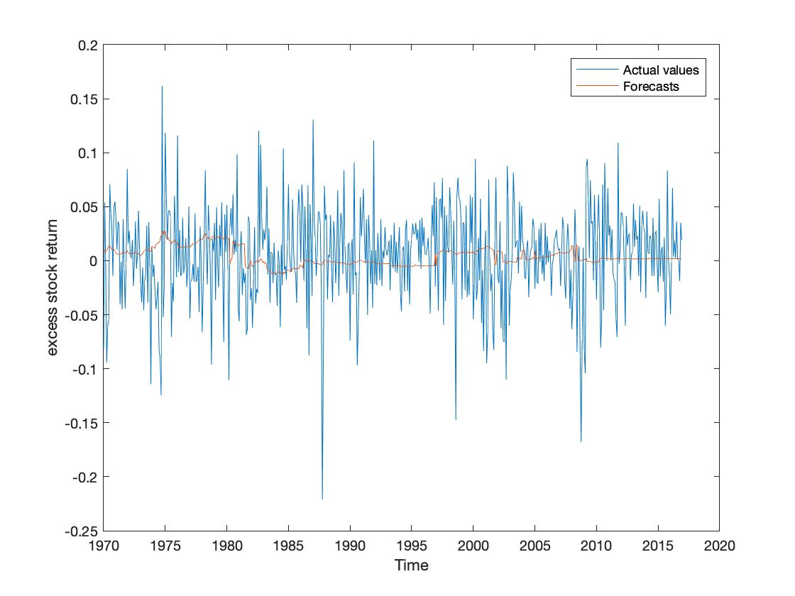
The root mean squared forecast error associated with the forecasts is 0.04515.

2.How often does your preferred model selection approach include different predictor variables?Forecasting代写

[hint: compute the average of the number of times that a predictor gets selected over the sample from 1970 through 2016].

The average of the number of times that the predictors get selected over the sample from 970 through 2016 are 0.0957, 0.7855, 0.0071, 0.0993, and 0.2145 for D/P, b/m, tbl, lty, and ntis, respectively. The other predictors are never selected.

3.Next,Forecasting代写

repeat the exercise when you use only a constantin the forecasting model. This is the prevailing mean (pm) model of Goyal and Welch and corresponds to a constant expected excess return. Again, compute the out-of-sample forecasts and the root mean squared forecast error from this model. Which produces the most accurate forecasts, your model in (1) or the prevailing mean model?

The plot of forecasts by pm model against the actual values is shown in below figure.

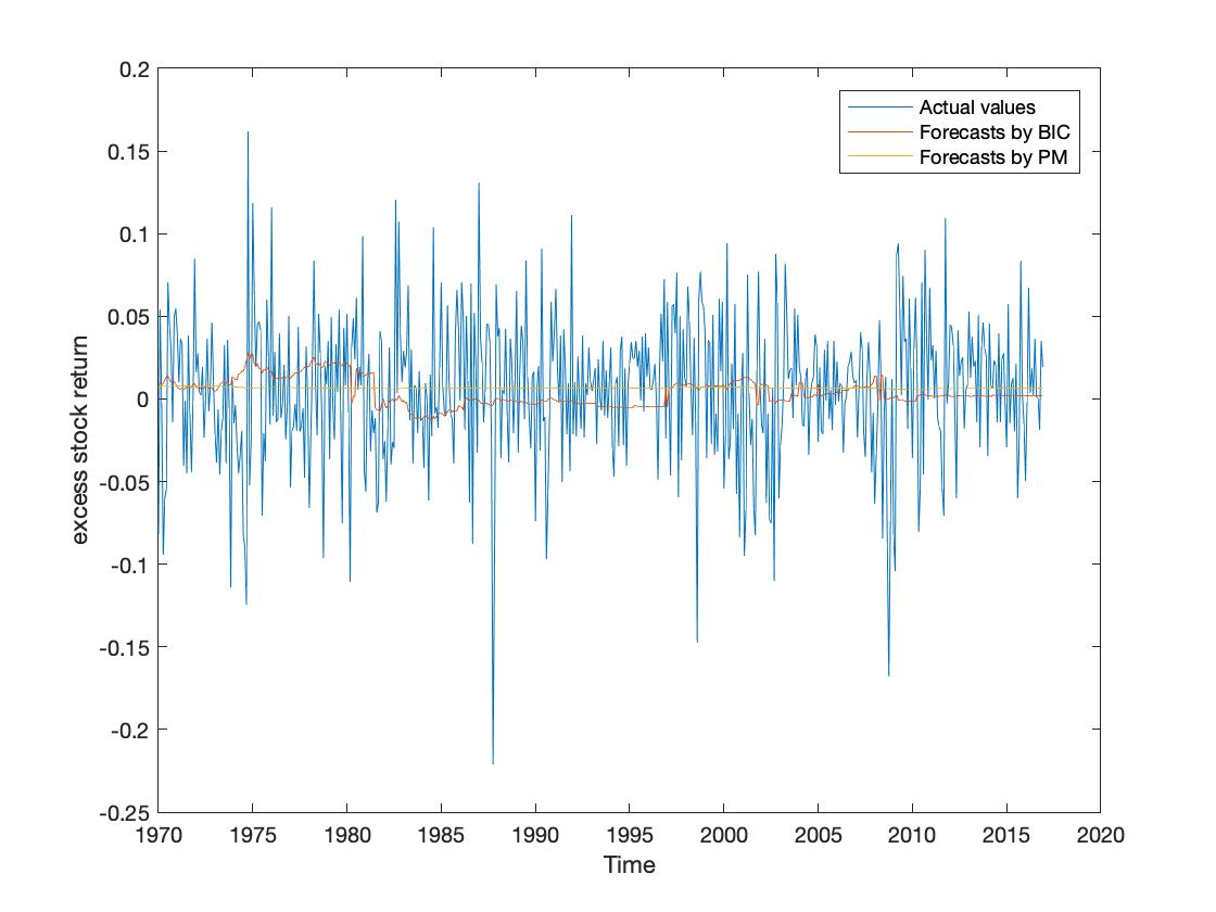
The root mean squared forecast error associated with the forecasts is 0.04409, which is less than the root mean squared forecast error in question 1. This implies that PM might be better for forecasting.Forecasting代写

4.Repeat the exercise

when you use the kitchen sink model that includes all 10 predictors (plus a constant). Plot the forecasts from this model and report the root mean squared forecast error. How well does this approach work?

The plot of forecasts by kitchen sink model against the actual values is shown in below figure.

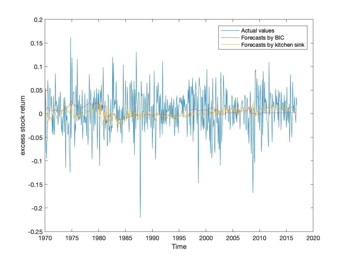
The root mean squared forecast error associated with the forecasts is 0.04520 which is larger than the root mean squared forecast error in question 1. This implies that PM might be worse for forecasting.

5.Replace the linear regression model

in (1) with a machine learning model of your choice such as a regression tree, LASSO, or a neural net. How well does your approach work for same out-of-sample period used in question 1?Forecasting代写

LASSO is performed. The plot of forecasts by LASSO against the actual values is shown in below figure.

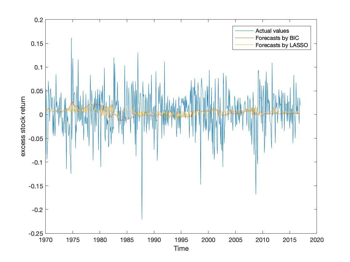The root mean squared forecast error associated with the forecasts is 0.04462, which is less than the root mean squared forecast error in question 1. This implies that LASSO might be better for forecasting.

Part II: Chinese travels

The excel file China_travels.xlsx contains monthly data on Chinese trips (in units of 10,000 trips) by rail (column B in the worksheet “travelers”) and by air (column C) over the period 1/1/2005 – 11/1/2018. The date of the Chinese New Year is contained in a separate worksheet (“Date of Chinese new year”). Also included in the worksheet “baidu search index” is the number of searches for air tickets (using different Chinese terms) in columns B, C and D along with searches for train tickets (column E) and intercity bus tickets (column F). These are daily data.

1.Does the daily search data help you predict monthly rail or plane trips?

Please report your preferred forecasting model and explains how/if it uses the Baidu search data. Make sure the search data is known prior to the month or which you are predicting the rail or plane trips (e.g., use September search data to predict October trips). You can use the full data sample up to 11/1/2018 to estimate your forecasting model.Forecasting代写

One may use the cumulative search counts for predicting the monthly trips by the model , where t is the month indicator and k = 4 for air trip prediction and k = 3 for rail trip prediction.

For air trip estimation, monthly cumulative search counts for variables air ticket 1,2, and 3 are used. For rail estimation, monthly cumulative search counts for variables train ticket and intercity bus tickets are used.

A dummy variable is introduced for indicating whether the Chinese New Year is in that month whose total trips is to be predicted for both air and rail prediction models.

The data up to 11/1/2018 is used for model training. The predicted air trips are 23989 and 22631 for December 2018 and January 2019, respectively. While the predicted rail trips are 42165 and 42241 for December 2018 and January 2019, respectively. Including the history information from the Baidu Index definitely increases the predictability.

合作平台：天才代写幽灵代写写手招聘 Essay代写