
Untitled
problem代写 Problem 1 – SAX method. Implement the SAX method in a programming language that you are comfortable with. Submit your code.

Your name
2018-11-16
Problem 1 – SAX method problem代写
Implement the SAX method in a programming language that you are comfortable with. Submit your code. The input is a time series and the output is a string.
data("economics")
glimpse(economics)

## Observations: 574
## Variables: 6
## $ date     <date> 1967-07-01, 1967-08-01, 1967-09-01, 1967-10-01, 1967...
## $ pce      <dbl> 507.4, 510.5, 516.3, 512.9, 518.1, 525.8, 531.5, 534....
## $ pop      <int> 198712, 198911, 199113, 199311, 199498, 199657, 19980...
## $ psavert  <dbl> 12.5, 12.5, 11.7, 12.5, 12.5, 12.1, 11.7, 12.2, 11.6,...
## $ uempmed  <dbl> 4.5, 4.7, 4.6, 4.9, 4.7, 4.8, 5.1, 4.5, 4.1, 4.6, 4.4...
## $ unemploy <int> 2944, 2945, 2958, 3143, 3066, 3018, 2878, 3001, 2877,...

changes <- diff(economics$pce)
changes_SAX <- SAX(changes, alphabet = 5, PAA = 30)
changes_SAX

##  [1] "b" "b" "b" "b" "b" "b" "b" "b" "c" "c" "c" "c" "c" "c" "c" "c" "c"
## [18] "c" "c" "d" "d" "c" "d" "e" "d" "b" "c" "d" "d" "d"
The economics is a dateset with 478rows and 6 variables. We the first order difference of pec(personal consumption expenditures) as a time series to propose SAX method. The alphabet_size set to 5 and Piecewise Aggregate Approximation equals to 30
Problem 2 – Regression problem代写
train <-  read.csv('blogData_train.csv', header = F)
test <- read.csv('blogData_test-2012.03.31.01_00.csv',header = F)

dim(train)

## [1] 52397   281

dim(test)

## [1] 214 281

# MSE function
MSE = function(y_hat, y) {
  mse = mean( (y - y_hat)^2)
  return(mse)
}

# Create model matrix for trainset and test set, basing on the dataset,we found the model matrix is really sparse.
train_x = model.Matrix(V281 ~ . - 1, data = train, sparse = F)
train_x_sparse = model.Matrix(V281 ~ . - 1, data = train, sparse = T)
train_y = train$V281

test_x = model.Matrix(V281 ~ . - 1, data = test, sparse = F)
test_y = test$V281

# LASSO to select variables

### using cv to select the best model
mdl_lasso = cv.glmnet(train_x_sparse, train_y, family = "gaussian", alpha = 1)
### calcluate our predict value on test set
pred_lasso = predict(mdl_lasso, newx = test_x)

# the MSE of LASSO regression
MSE(pred_lasso, test_y)

## [1] 1768.295
Using blogDate_test-2012.03.31.01_00.csv as train set, we propose a LASSO regression on it. Basing on CV method to select a best model. The MSE on test set is 1853.85.
Problem 3 – Weka and Apriori problem代写
the top 10 rules found with confidence above 0.8
- biscuits=t frozen foods=t fruit=t total=high 788 ==> bread and cake=t 723 <conf:(0.92)> lift:(1.27) lev:(0.03) [155] conv:(3.35)
- baking needs=t biscuits=t fruit=t total=high 760 ==> bread and cake=t 696 <conf:(0.92)> lift:(1.27) lev:(0.03) [149] conv:(3.28)
- baking needs=t frozen foods=t fruit=t total=high 770 ==> bread and cake=t 705 <conf:(0.92)> lift:(1.27) lev:(0.03) [150] conv:(3.27)
- biscuits=t fruit=t vegetables=t total=high 815 ==> bread and cake=t 746 <conf:(0.92)> lift:(1.27) lev:(0.03) [159] conv:(3.26)
- party snack foods=t fruit=t total=high 854 ==> bread and cake=t 779 <conf:(0.91)> lift:(1.27) lev:(0.04) [164] conv:(3.15)
- biscuits=t frozen foods=t vegetables=t total=high 797 ==> bread and cake=t 725 <conf:(0.91)> lift:(1.26) lev:(0.03) [151] conv:(3.06)
- baking needs=t biscuits=t vegetables=t total=high 772 ==> bread and cake=t 701 <conf:(0.91)> lift:(1.26) lev:(0.03) [145] conv:(3.01)
- biscuits=t fruit=t total=high 954 ==> bread and cake=t 866 <conf:(0.91)> lift:(1.26) lev:(0.04) [179] conv:(3)
- frozen foods=t fruit=t vegetables=t total=high 834 ==> bread and cake=t 757 <conf:(0.91)> lift:(1.26) lev:(0.03) [156] conv:(3)
- frozen foods=t fruit=t total=high 969 ==> bread and cake=t 877 <conf:(0.91)> lift:(1.26) lev:(0.04) [179] conv:(2.92)
maximum minimum-support
c <- seq(0.1, 0.9, by = 0.1)
max_minsupport <- c(.45, .45, .45, .45, .45, .45, .4, .3, .15)

plot(c,max_minsupport,type = 'l')
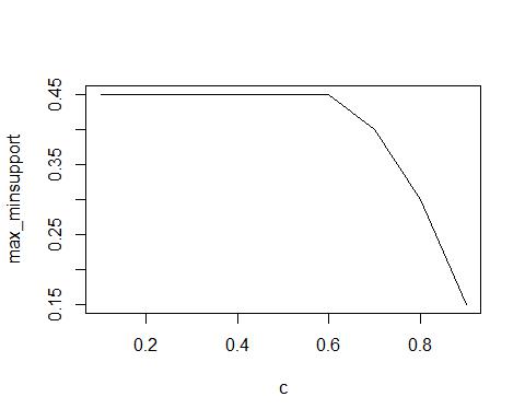
We set c = c(0.1,0.2,…,0.9), run the model to get maximum minimum support. We observed that maximum minimum-support decreses with increasing confidence values. problem代写

更多其他:app代写 assignment代写 C++代写 CS代写 作业加急 作业帮助 加拿大代写 北美cs代写 北美代写 北美作业代写 数据分析代写
