金融非线性计量经济学代写

Nonlinear econometrics for finance – Homework 3

 

金融非线性计量经济学代写 In the first p art o f t he h omework you w ill e stimate t he C onsumption C APM u sing G MM. I n t his appli- cation

 

In the first p art o f t he h omework you w ill e stimate t he C onsumption C APM u sing G MM. I n t his application, we estimate the model with monthly data on consumption growth and returns, and we will make useof instrumental variables estimation. Remember that in the first h omework, for the linear regression model,you have shown that when the errors ε_t are correlated with the regressors x_t, you can use a set of additionalvariables z_t uncorrelated with the error term ε_t, but possibly correlated with the regressors x_t to re-establish consistency of your estimated coefficients β.金融非线性计量经济学代写

The same is possible with nonlinear models, and nonlinear errors. The first q uestion o f t he h omework w ill g uide you t hrough t he a pplication o f i nstrumental variables in a nonlinear model, the C-CAPM. The data to use for Question 1 are in the file ccapmmonthlydata.xls.

In the second part of the homework, you will estimate extensions of the GARCH(1,1) model we have discussed in class using the maximum likelihood estimator (MLE). In particular, you will estimate a GARCH- M model and a T-GARCH model. Please read the slides of Lecture 6 carefully and practice with the code that I have provided for estimation of the traditional GARCH model. You should use the S&P500 data for Question 2.

1 Question 1 (50 points) 金融非线性计量经济学代写

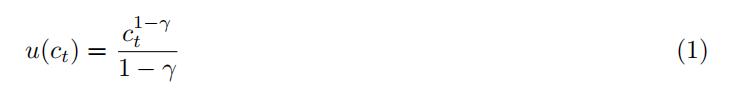
Consider the same C-CAPM model described in class, with CRRA utility function

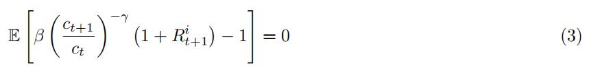
We have shown in class and in the second homework that the model provides the following conditions for all time periods t = 1, 2, …, and all assets i = 1, 2, …, N

This provides a system of equations – one per asset – that we can use to estimate the parameters β and γ. Indeed, the conditions in (2) are valid for any period t, and using the law of iterated expectations we can write the unconditional expectation

The GMM estimator solves the system of equations in (3) to find the parameter estimates for β and γ.

During the lectures, we also noticed that we can use equation (2) to create new moments conditions. Wehave done this with the diffusion models in class, but the same logit applies here. Indeed, if we multiply theconditional moment equation (2) by a function of variables contained in the information set of the investor, we can obtain new moment conditions. To be concrete, remember that the notation E_t means

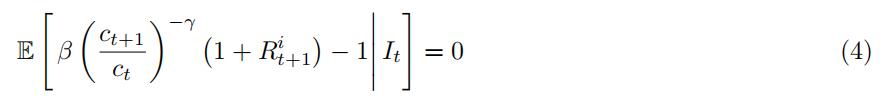
where I_t is all the information available for the inverstor at time t. This information includes past values of consumption growth and returns,

This means that if we multiply any variable that is part of the information set I_t by one of the moment conditions, the equation will still be equal to zero. The reason is that anything in the information set at time t is a constant when computing the expected value at time t. Concretely, consider the moment condition

This is always true as we are multiplying by a conditional expected value that we know is equal to zero.金融非线性计量经济学代写

That means that if we take  inside the expected value we still have an expected value equal to zero.

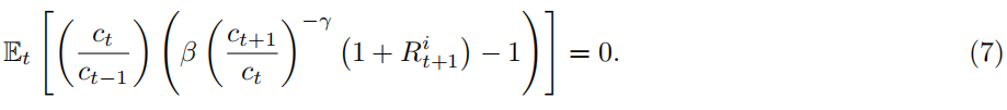
If this is the case, then the equation (7) is satisfied for any t and using the law of iterated expectations we can use the unconditional moment condition

as an additional moment to estimate our parameters.金融非线性计量经济学代写

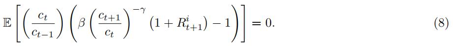
This means that now for each asset i = 1, …, N we have two moment conditions to use for estimation

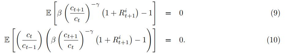
for a total of 2N moment conditions.

Notice how this is analogous to what we saw in the first homework with instrumental variables.金融非线性计量经济学代写

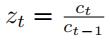
Indeed, we think of  as an instrumental variable:

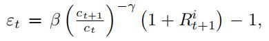
• is uncorrelated with the error in our nonlinear equation

  

because we have just shown

because we know that E (ε_t) = 0.

• is correlated with the data, since it is certainly correlated with consumption growth in the next period

  

Data description The data in the file ccapmmonthlydata.xls are monthly data on consumption growth and asset returns from February 1959 to November 1993 (not quarterly as in the first homework). The  first column contains the date; the second column contains the time series for the consumption growth .金融非线性计量经济学代写

Columns 3-13 are your asset returns for 11 assets.

4. (10points) Estimate the model using the usual moment  This is equivalent to what you did in Homework 2 with the quarterly data. Please use the HAC estimator for the standard errors. (HINT: note that the data contains consumption growth  for t = 1, …, T and not consumption levels c_t for t = 1, …, T . Modify the code from homework 2 accordingly, to compute the moments correctly.)
5. (5points) Perform the Hansen test for overidentifying restrictions for this  Explain your result.金融非线性计量经济学代写
6. (20 points) Use the lagged consumption growth  as your instrumental This means that you need to add N moments to the usual moment conditions you used in the previous estimation. Re-estimate the model using all the moment conditions (the original N moments and the new instrumental variable moments). Please use the HAC estimator for the standard errors. Are your results different from the estimates obtained in the first question? Why?
7. (5points) Perform the Hansen test for overidentifying restrictions for this new  Explain your result.
8. (10 points) Is there any other variable that you  could use as instrumental variable?  Explain why  and write the moment conditions that you would use for estimation. (You don’t need to perform the estimationin Matlab for this last question).

2 Question 2 (50 points) 金融非线性计量经济学代写

1. (10points) Estimate a GARCH(1,1)-M model using the Maximum Likelihood Estimator (see slides of Lecture 6 for details on the model):

r_t = βh_t + ε_t,

ε_t = √h_tu_t, with E_t−1(u_t) = 0 and E_t−1(u²) = 1

h_t = µ^∗ + δ^∗h_t−1 + φ^∗ε² .

2. (10points) Compute standard errors (not using the gradient function in Matlab).
3. (4 points) Test whether the parameter β is significant. Test whether β =5.
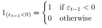
4. (8 points) Estimate a T-GARCH(1,1) model using the Maximum Likelihood Estimator (see slides of Lecture6 for details on the model):

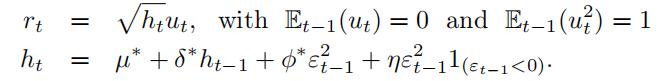
where 1_(εt−1<0)  is a variable that is equal to 1 when ε_t−1 < 0 and it is 0 otherwise

5. (10points) Compute standard errors (not using the gradient function in Matlab).
6. (2 points) Test if the parameter η is signifificant.
7. (6 points) Plot the time series of conditional variances in both cases. Do you see anything interesting in some timeperiods?

其他代写：代写CS C++代写 java代写 r代写 matlab代写 web代写 app代写 金融经济统计代写 作业代写 物理代写 数学代写 考试助攻

合作平台：essay代写 论文代写 写手招聘 英国留学生代写