
Take-Home Exam #2:
金融考试代写 Your handout should consist in two main outputs:1.A well-written and well-presented report, detailing your procedure to obtain the needed
Estimating the risk premia with standard models
G.Roussellent
Winter 2019 – Due: March 30th, 11:59pm

Introduction 金融考试代写
Your handout should consist in two main outputs:
- A well-written and well-presented report, detailing your procedure to obtain the needed results and commenting on the results when
- For R-users, one well-commented and indented script containing all functions and commandlines to obtain your results, including lines generating For Excel-users, one Excel le containing the collection of spreadsheets that you needed to obtain your results and graphs. Both R and Excel les should work on any computer!
If you are using results from the class, please detail them in your report. If you are using results from external sources, please create a proper bibliography in your report.
Preamble 金融考试代写
Download the data corresponding to your group number on your computer.
In this problem, we explore the risk premium implications of a standard model one-factor pricing model. This model is the discrete-time equivalent of Vasicek’s (1977) seminal model. In the rst part, we see which assumptions we need to obtain time varying risk premium on bonds. We also show that this model proves limited in several dimensions, especially in tting the yield curve at each point in time.
In the second part, we try to x these issues by considering a model where a new factor is introduced. After providing economic interpretation for this factor, we show how it can easily correct for some of the undesirable features of the one-factor model. We nally obtain risk premium estimates during the crisis that we can interpret economically.金融考试代写
Although the problem looks long,
each question can be answered in a very quick fash- ion. They usually boil down to very simple computations and plots. The important part is to cleanly interpret the results we are obtaining, such that we really understand where the crucial assumptions lie.
A signi cant amount of questions require showing results with pen and paper. Although some of you are familiar with math-typing in Word or in LATEX, I understand it is not the case for all of you. I thus accept cleanly written manuscript pages scanned as part of your report.
1 Implications of a simple one-factor model (65%)金融考试代写
Let rt = rt(1/12) be the one-month maturity yield of a sovereign zero-coupon bond. Without abuse, we will call this the short-term interest rate. We drop the brackets for notational convenience. We assume that the risk-neutral dynamics of rt are given by:
rt = µ∗ + ρ∗(rt−1 − µ∗) + σε∗t , where ε∗t ∼ N (0, 1) . (1) We can show that in this case (see Appendix A.1), the yield curve is given by:
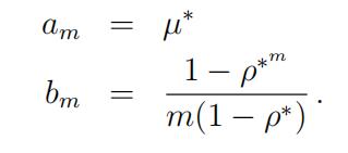
rt(m) c am + bm × (rt − µ∗) , (2) where m is expressed in months (m = 12 for the 1y maturity), and:
1.In this part, we explore the implications of this pricing formula for chosen parameters. (20%)financial1代写
(a)Whatdo the parameters µ∗ and ρ∗ represent? Provide their names and explain why am = µ∗. (1% )
(b)Computethe loadings bm for all monthly maturities ranging from 1-month to 20
years (240 maturities), using successive values ρ∗ = 0.5, ρ∗ = 0.9, ρ∗ = 0.99. Plot the 3 resulting curves on the same graph and comment on the impact of ρ∗ on the yield curve. (3% )金融考试代写
(c)Provided your answer to the previous question, explain when the yield curve will be upward sloping and when it will be downward Provide the economic mechanism underlying this result. (2%)
(d)Plotthe yield curve for rt = 3%, µ∗ = 4% and ρ∗ = 0.9. What would happen if
µ∗ = 3%? Explain. (2% )
(e)Showwith pen and paper that the excess returns of holding the bond of maturity m for h months is given by: (6% )
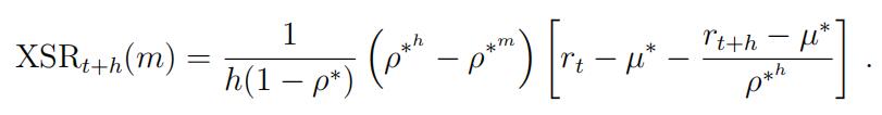
(f)Provided ρ∗(0, 1), express the condition on the short-term yield variation such that the excess returns are If ρ∗ grows closer to one, how is this condition a ected? Explain the economic mechanism underlying this result. (2% )金融考试代写
(g)Assume that the true (by opposition to risk-neutral) average of the short-rate is 3%. Compute the average excess returns for m = 12, 60, 120 , h = 12, 24, 60, ρ∗ = 0.5, 0.9, 0.99 , and µ∗ = 2%, 3%, 4% . Provide your results in a Table.(4% )
2.Now we consider that the true dynamics of the short-rate is givenby:
rt = µ + ρ (rt−1 − µ) + σεt, where εt ∼ N (0, 1) . (5)
We explore what happens on the risk premium for di erent choices of µ and ρ param- eters. (20%)
(a)Show with pen and paper that the yield that would be obtained under the expec- tation hypothesis if given by:
r(EH)(m) = a(EH) + b(EH) × (rt − µ) ,
and provide the formulas for a(EH) and b(EH). (2% )金融考试代写
(b)Consider rst that ρ = ρ∗. The only di erence between the true and the risk- neutral dynamics thus lie in the di erence from µ to µ∗. Do you expect µ to be larger or smaller that µ∗? Explain your intuition. (1%)
(c)Show with pen and paper that the risk premium in this model depends on the maturity but does not vary over Is the risk-premium increasing ordecreasing with maturity? (3% )
Hint: remember that the risk premium is de ned by RPt(m) = rt(m) − r(EH)(m).
(d)Show with pen and paper that the expected excess returns in this model aregiven
by:
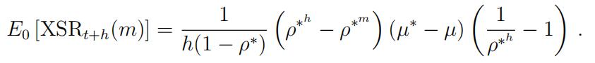
Comment the relationship between expected excess returns and µ∗ µ. Is this what you expect? (6% )
Hint: Remember that E0(rt+h) = µ + ρh(rt − µ).
(e)Set µ∗− µ = 1%. Provide the two following plots which represent 3 curves, for
ρ∗ = {0.5, 0.9, 0.99}:
i.plotthe expected excess returns for h = 12 and m is on the x-axis.金融考试代写
ii.plotthe expected excess returns for m = 120 and h is on the x-axis.
Comment on the in uence of the persistence ρ∗, of the maturity of the bond m
and the holding period h on the expected excess returns. (2% )金融考试代写
(f)We now consider that ρ∗> ρ. Explain why this relationship makes sense from an economic standpoint. (2% )
Hint: a high persistence means that the shocks tend to have an in uence for a longer time. In essence they last longer .
(g)Redo questions (c-e) considering for question (e) that ρ = ρ∗− 0.05 and that rt = 3%. How do the expected excess returns vary with rt? Interpret this relationship.
(6% )
Hint: the resulting expected excess returns are now given by:

3.Now that we have explored the theory underlying this model, we are interested in backing out the parameters from the data.(25%)
(a)Compute the average of the 1-month yield. Explain why this procedure gives you anestimate for µ and provide its value µˆ. (2% )金融考试代写
(b)Formthe demeaned series of the 1-month yield (rt µˆ) and regress it on its own Explain why this gives you an estimate for ρ and provide its value. (2% )
(c)Compute the R2from the regression and comment on the quality of the AR(1) model under the true probability measure. (2% )
Hint: Remember that the R2 is given by one minus the ratio of the variance of the residuals divided by the variance of the dependent variable.
(d)Toestimate the risk-neutral parameters µ∗ and ρ∗, form the series of yields implied by the model as a function of the parameter µ∗ and ρ∗, for each maturity that you observe in the Estimate the parameters by minimizing the sum of squared residuals between the observed and the model yields. (5% ), (µ∗ and ρ∗ do not depend on time, so you only back out one value for each of these for the entire time series.)
(e)For each date in the sample, compute the R2of how the model ts the yield curve. Represent the time series of the R2 and explain the good/bad tting properties of the model. (6% )金融考试代写
(f)Compute the time series of the term-premium for each maturity and represent them on a plot. Comment on its evolution during the crisis.(4% )
(g)Use the estimated parameters to compute the expected excess returns of holding the longest-maturity bond for one year. Compare the expectation to the realized excess returns (with a R2measure for instance). Comment on the quality of the model. (4% )
2 Improving the quality of the model (35%)
One of the key reasons why the tting quality of the model is poor is that the exibility of the model under the risk-neutral measure is too limited. Indeed, in the one-factor case, the slope of the curve is strongly related to where the current short-rate is with respect to its long-run mean. This section introduces a model to solve this issue.
We consider the following model under the risk-neutral measure:
where µt is not observable. We can show (see Appendix A.2) that the yield curve is given by:
rt(m) = am + bm × (rt − µ∗t ) + cm × (µ∗t − µ∗) . (7)
The coe cients are now given by:
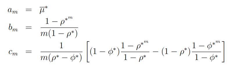
1.In this part, we try to get an understanding of the new formulation of this model. (15%)
(a)Explainwhy this new formulation makes sense with respect to the issues observed for the one-factor model. What do you expect in terms of t for this new model? (2% )
(b)Compute the loadings cmfor all monthly maturities ranging from 1-month to 20 years (240 maturities), using successive values ρ∗ = 0.5, ρ∗ = 0.9, ρ∗ = 0.99, and
φ∗ = 0.45, φ∗ = 0.88, φ∗ = 0.97. Present your results as three plots, one for each
value of ρ∗. Each plot will contain 3 curves, corresponding to each value of φ∗. x-axis is the maturity. Comment on the impact of φ∗. (5% )
(c)Providea methodology to back out the time series of µ∗t given an assumed value for µ∗, ρ∗, and φ∗. (3% )
Hint: Try to reformulate the model as a linear regression framework.
(d)Provide a methodology to estimate µ∗, ρ∗, and φ∗. (2%)
(e)Estimate the parameters of the model. Provide the time series of the R2and the time series of the estimated µ∗t on two di erent Compare the R2 to the ones obtained in the rst section. Try to provide justi cation for the movements of µ∗t . (3% )
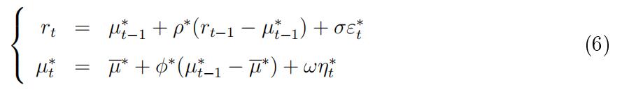
2.Assumethat the model under the true measure is given by:
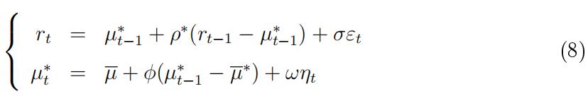
that is, the only di erence lies in the parameters driving the dynamics of µ∗t . (20%)
(a)Doyou expect µ to be larger or smaller than µ∗? Same question with
φ∗ and φ. (2% )
(b)Show with pen and paper that the yield that would be obtained under the expec- tation hypothesis if givenby:
r(EH)(m) = a(EH) + b(EH) × (rt − µ∗) + c(EH) × (µ∗ − µ) ,
and provide the formulas for a(EH), b(EH) and c(EH). (2% )
(c)Given your result to the previous question, show that the term premium only movesover time because of the time-variation of µ∗t . (4% )
(d)Similarly to the method developed in the rst part, estimate µ with a simple average and φ with a simple regression. (5%)
(e)Compute and plot the term structure of the term premium. Compare to what you obtained in the rst part. Comment on its evolution during the crisis. Do you reach di erent conclusions than in the rst part? (7%)
A Appendix
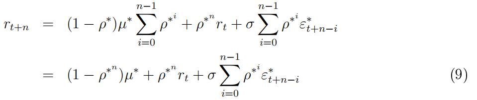
A.1 Solving the one-factor model
Starting from Equation (1), we have:
rt+n = µ∗ + ρ∗(rt+n−1 − µ∗) + σε∗t+n
= (1 − ρ∗)µ∗ + ρ∗rt+n−1 + σε∗t+n
= (1 − ρ∗)µ∗ + ρ∗ (1 − ρ∗)µ∗ + ρ∗rt+n−2 + σε∗t+n−1 + σε∗t+n
= (1 − ρ∗)(1 + ρ∗)µ∗ +
Iterating, we obtain:
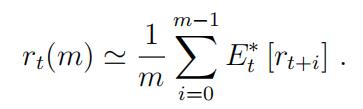
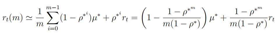
Let us work through our the approximate pricing formula. We know that:
Using the fact that all shocks ε∗t are mean zero, we have:
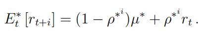
Thus, we obtain:
A.2 Solving the two-factor model
We start back from Equation (8). Let us call Xt = (rt, µ∗t )j. We express the model in matrix form:
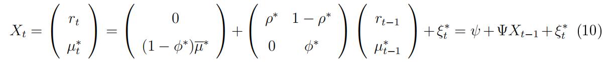
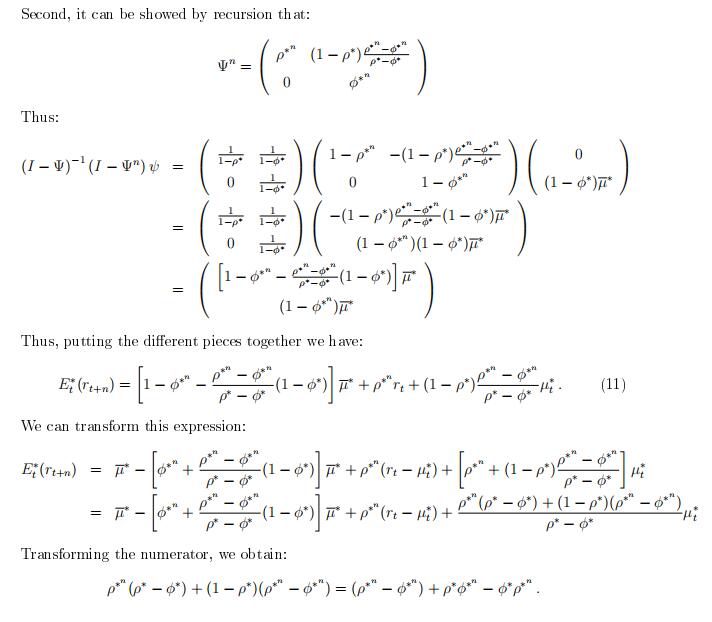
We need to compute the best forecast of the short-term interest rate. We can show by recursion that:
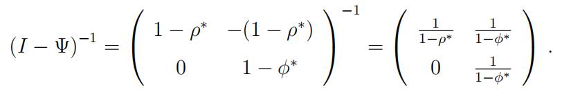
E∗ [Xt+n] = (I − Ψ)−1 (I − Ψn) ψ + ΨnXt .
Let us compute each of these terms. First:
Doing the same for the term in µ∗, we obtain:
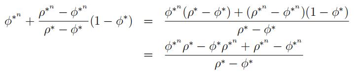
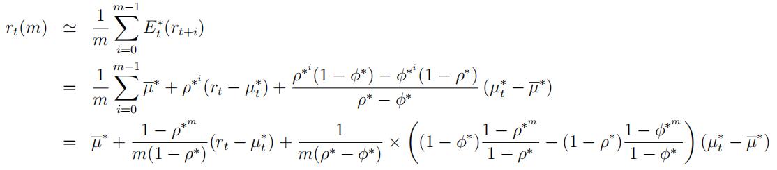
Thus, we eventually obtain:
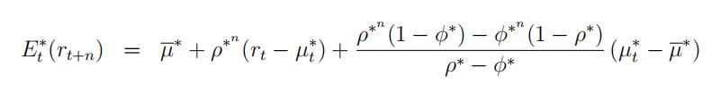
The yield at maturity m is approximately given by the average of risk-neutral forecasts of future short-term yields. Hence:

其他代写:java代写 function代写 web代写 编程代写 report代写 数学代写 algorithm代写 python代写 java代写 code代写 project代写 代码代写 dataset代写 analysis代写 C++代写 代写CS 金融经济统计代写 essay代写 assembly代写 program代写
