Coursework代写 Energy Analytics代写 Built Environment代写

MSc ESDA Coursework Title Page

Coursework代写 UCL Candidate Code: ZFGM1Module Code: BENV0092Module Title: Energy Analytics in the Built Environment Coursework Title: The

UCL Candidate Code: ZFGM1

Module Code: BENV0092

Module Title: Energy Analytics in the Built Environment Coursework代写

Coursework Title: The effects of dwelling energy efficiency interventions on gas consumption in the UK: A comparison by dwelling characteristics

Module Leader: Despina Manouseli

Date: 07/01/2019

Word Count: 2,997

By submitting this document, you are agreeing to the Statement of Authorship: Coursework代写

I/We certify that the attached coursework exercise has been completed by me/us and that each and every quotation, diagram or other piece of exposition which is copied from or based upon the work of other has its source clearly acknowledged in the text at the place where it appears.

I/We certify that all field work and/or laboratory work has been carried out by me/us with no more assistance from the members of the department than has been specified.

I/We certify that all additional assistance which I/we have received is indicated and referenced in the report.Coursework代写

Please note that penalties will be applied to coursework which is submitted late or which exceeds the maximum word count. Information about penalties can be found in the MSc ESDA Course Handbook which is available on Moodle:

• Penalties for late submission:https://moodle-1819.ucl.ac.uk/course/view.php?id=9967&section=30

• Penalties for going over the word count:https://moodle- 1819.ucl.ac.uk/course/view.php?id=9967&section=30

In the case of coursework that is submitted late and is also over length, then the greater of the two penalties shall apply. This includes research projects, dissertations and final reports.

The effects of dwelling energy efficiency interventions on gas consumption in the UK: A comparison by dwelling characteristics

1. Introduction

Almost one fourth (434 TWh) of the total final energy in the UK is consumed to meet heating requirements in households (Ofgem, 2016). Additionally, 17% of UK’s CO2 emissions were generated by the residential sector in 2017 (UK BEIS, 2018). With a growing population living in smaller families, how can the goal to reduce CO2 emissions related to domestic heating by 80% in 2050, as committed in the 2008 Climate Change Act, be achieved?

While heat decarbonization technology (e.g. hydrogen, mechanical heat pumps, heating districts) still remains on experimental deployments, and considering UK’s building stock characteristics, energy efficiency is by far the most prioritized strategy to address fuel poverty, optimize energy consumption and reduce CO2 emissions.

Naturally,

each type of energy efficiency interventions has a different impact in energy consumption depending on the dwelling characteristics like property type, age, location, and size. Therefore, it is relevant from a public policy perspective to quantify the effects of energy efficiency measures, distinguishing between the spatial characteristics of the dwelling, in order to optimally target energy efficiency programs.

The following document presents a quantitative analysis of the effects of energy efficiency interventions, done on dwelling fabric and services, over gas consumption on households in the UK. While presenting significant evidence of the effects of cavity wall insulation, loft insulation and boiler replacements, the document also includes a comparative analysis of the effects of the interventions by the following dwelling spatial characteristics: property age, floor size, property type and location (region).

2. Literature review

Energy efficiency in the built environment has been a relevant research area considering the potential impact on reducing GHG emissions. As stated by (Anderson, Wulfhorst and Lang, 2015) the assessment on built environment has been done from an individual building perspective (Doukas, Nychtis and Psarras, 2009; Heo, Choudhary and Augenbroe, 2012; Asadi et al., 2014) or from an urban level (Haines et al., 2009; Heinonen, Kyrö and Junnila, 2011).

Understanding the determinants of energy consumption has therefore also been a relevant research topic, and with the recent development of advanced metering infrastructure the friction of accessing data has been removed (Zhou and Yang, 2016). (Jackson and Druckman, 2008) demonstrate the importance of socio-

economic factors in household energy consumption,

(Guerra-Santin and Itard, 2010; Frederiks, Stenner and Hobman, 2015) highlight the relevance of occupants behavior in domestic energy consumption. In contrast, other authors feature dwelling characteristics as the most relevant driver of energy consumption (Braun, 2010; Aksözen et al., 2015). (Huebner et al., 2015) find that building variables explained 39% of the variability in household energy consumption in the UK.

Energy efficiency interventions have been largely deployed worldwide. (Hamilton et al., 2014) find that in the 2000-2007 period 9.3 million dwellings (40%) in England had an energy efficiency measure installed. While some authors address the barriers to energy efficiency measures adoption (Crosbie and Baker, 2010; Gillingham, Newell and Palmer, 2010; Pelenur and Cruickshank, 2012; Scott, Jones and Webb, 2014), other focus in finding determinants to explain the energy efficiency gap -the difference between actual impact and potential impact- (Brounen, Kok and Quigley, 2012; Van Den Brom, Meijer and Visscher, 2018).

Regarding the assessment of the impact energy efficiency interventions,

one approach consists in modelling the physical equations of the property and calculating the effect of the intervention (Battista et al., 2014; Steemers and Ben, 2014). One the other hand, methodologies that use empirical field evidence to quantify the effect of the energy efficiency interventions is a more widely used approach (Brounen, Kok and Quigley, 2012; Dall’O’, Galante and Pasetti, 2012; Adan and Fuerst, 2016; Fowlie, Greenstone and Wolfram, 2018).

(Hamilton et al., 2013) propose Energy Epidemiology as new approach to end-use energy demand research. As an analogy to the health sciences discipline, energy epidemiology is a research framework based on the use empirical evidence to understand the heterogeneity of factors that lead to certain end-use energy related outcome. Regarding interventional studies, energy epidemiology suggests the need of consider different factors, including dwelling characteristics, in order to assess the effectiveness of certain energy efficiency intervention.

Finally the use of econometrics techniques to measure the effect of energy interventions are widely use. Particularly, to conduct analysis over empirical evidence comparing control and treatment groups. Specifically panel data analysis, that involve both temporal and cross-sectional data variations, have been used to explain energy consumption at a macro level (Lee, 2005; Wang et al., 2011).

3. Data and methodology Data

The data source1 used for the proposed analysis is the National Energy Efficiency Data-Framework (NEED). NEED is a government-administrated2 dataset of

1 Available in: https://www.ukdataservice.ac.uk/

2 Provided by UK BEIS

households in the UK that matches energy consumption data (gas and electricity), with information on energy efficiency measures installed, and data about dwelling characteristics.

The NEED dataset was filtered to observations households that had gas consumption between 3,000 and 50,000 kWh-year and electricity consumption between 100 and 25,000 kWh-year (Adan and Fuerst, 2016). Similarly, households with yearly change in gas consumption larger than 75% in absolute value are considered outliers and ignored from the analysis. Only household with complete information for the whole period of analysis were considered in order to have a balanced data panel. The resulting input dataset considers 22,826 households. Additionally, in order to consider the effect of weather in gas consumption, average yearly temperature data by region is sourced from the Met Office3.

Gas consumption and temperature,

which are the only temporal variables, range from 2005 to 2012. Cross section time-invariant household variables related to dwelling characteristics are: property type, property age, floor size and region. Three different type of energy efficiency interventions and considered4: Cavity wall insulation, loft insulation and boiler replacement. Table 1 summarize the number of household by dwelling characteristics and type of intervention.

Table 1. Dataset household count by intervention type (WI: Wall Insulation, LI: Loft insulation, B: Boiler replacement) and dwelling characteristics.

Region	none	WI	LI	B	WI&LI	WI&B	LI&B	WI&LI&B	total
all	10,305	2,043	2,196	3,872	1,536	930	1,185	769	22,836
East of England	1,207	211	208	433	130	85	111	70	2,455
London	1,611	90	205	604	31	44	95	16	2,696
Midlands	1,736	363	473	727	298	174	255	155	4,181
North East	399	188	135	167	152	83	88	77	1,289
North West	1,162	370	339	379	303	159	155	127	2,994
South East	1,840	336	256	707	229	149	148	113	3,778
South West	890	192	194	339	142	95	98	85	2,035
Wales	520	98	142	145	95	23	91	33	1,147
Yorksh. and Humber	940	195	244	371	156	118	144	93	2,261

Dwelling type	none	WI	LI	B	WI&LI	WI&B	LI&B	WI&LI&B	total
all	10,305	2,043	2,196	3,872	1,536	930	1,185	769	22,836
Bungalow	839	299	294	386	274	178	197	155	2,622
Detached	1,885	414	351	645	307	158	191	145	4,096
End terrace	1,026	184	211	389	141	89	145	66	2,251
Flat	1,090	111	48	415	21	66	34	12	1,797
Mid terrace	2,402	238	583	835	186	101	242	93	4,680
Semi-detached	3,063	797	709	1,202	607	338	376	298	7,390

3  Available in: https://www.metoffice.gov.uk/climate/uk/summaries/datasets

4 The combination of interventions is also considered

Year built	none	WI	LI	B	WI&LI	WI&B	LI&B	WI&LI&B	total
all	10,305	2,043	2,196	3,872	1,536	930	1,185	769	22,836
before 1930	2,943	127	683	1,060	95	60	296	47	5,311
1930-1949	1,736	358	443	720	278	177	232	162	4,106
1950-1966	1,605	676	407	718	500	317	234	224	4,681
1967-1982	1,767	578	394	769	478	272	267	249	4,774
1983-1995	1,186	204	219	401	157	91	138	78	2,474
1996 onwards	1,068	100	50	204	28	13	18	9	1,490

Floor size	none	WI	LI	B	WI&LI	WI&B	LI&B	WI&LI&B	total
all	10,305	2,043	2,196	3,872	1,536	930	1,185	769	22,836
1 to 50	667	77	41	266	26	50	40	11	1,178
101-150	3,482	678	733	1,226	544	277	384	250	7,574
51-100	5,305	1,184	1,247	2,075	903	564	683	472	12,433
Over 151	851	104	175	305	63	39	78	36	1,651

Methodology

Considering the availability of cross section and time series data, the proposed methodology to assess the effect of energy efficiency interventions in gas consumption is the econometric technique of panel data analysis. The methodology assumes the dependent time series variable can be explained by heterogenic characteristics proper to the individual that may vary in time (Wooldrige, Jeffrey, 2011). Panel data is widely used in different fields to understand the dynamics of change.

The proposed model is explained by the following linear equation:

Where 𝑖 = 1,2, … , 𝑁 represents each household in the dataset, 𝑡 = 1,2, … , 𝑇 refers to the time period, 𝐺𝐶 is yearly gas consumption in kWh, 𝑇𝐸 is the temperature difference relative to the previous year in degrees Celsius, 𝐼_𝑊𝐼, 𝐼_𝐿𝐼 and 𝐼_𝐵 are dummy variables (0 or 1) that indicate respectively if a cavity wall insulation, a loft insulation or a boiler replacement took place in that specific year. 𝛼, 𝛿, 𝜌, 𝛽1, 𝛽2 and 𝛽3 are the regression coefficients subject to estimation and 𝑒 is the error term.

Is relevant to highlight that the error term in the proposed model variates within individuals and by time.

In the panel data framework this estimation variation is called random effects. As opposed to fixed effects, where the error term is fixed for each individual, random effect modelling is used in this analysis to consider the fact that the dataset is a sample of larger population of households and therefore the interest is to estimate the general variability within all households rather than effect of individual households.

Parameters 𝛽1, 𝛽2 and 𝛽3 are interpreted as the effect in absolute terms (kWh) that cavity wall insulation, loft insulation and boiler replacement respectively have on gas consumption. In the other hand, since 𝑇𝐸 is temperature difference, 𝜌 is interpreted as the effect in absolute terms (kWh) that a change of one degree Celsius of the average yearly temperature has on gas consumption.

With the model defined by the previous equation,

the methodology to include dwelling characteristics in the analysis is the comparison of parameters estimates (𝛼, 𝛿, 𝜌, 𝛽1, 𝛽2 and 𝛽3) between each group. In that sense, the data set is filtered by every possible instance of each dwelling characteristic (e.g. properties in London) and sequentially the panel data parameters estimates are calculated and compared. As noted in table 1, the four dwelling features derive in 25 different dwelling characteristics, therefore 25 different models are estimated. With the parameter estimation for each group, the results are compared and analyzed.

The parameter estimation technique of the panel data with random effects is generalized least squares. The computational implementation is done in R with the plm package (Croissant and Millo, 2008).

4. Analysis and results

Figure 1 presents the difference in gas consumption by all the possible combinations of interventions considered. As expected, it results evident that the average gas consumption of the group of dwellings without any interventions is the highest. In the other hand, there is no clear assessment on which of the intervention is most effective.

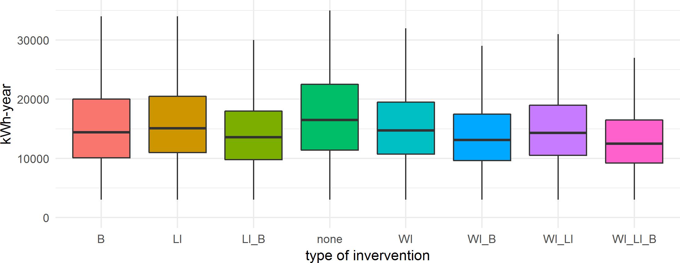
Figure 1. Average household gas consumption by type of intervention (WI: Wall Insulation, LI: Loft insulation, B: Boiler replacement).

To answer this,

the proposed model estimation was conducted with all the dwellings in the dataset, the results are summarized in Table 2. With this model, 82% of the variance in gas consumption is explained (r-squared) and all the estimates are statistically significant at a 95% confidence level.

Table 2. Model estimation results with all the data

	Estimate	Std. Error	t-value	p-value
α	1,320	20.69	63.8	0
δ	0.88	0.001	851.6	0
ρ	-301	9.10	-33.1	7.10E-240
β1 (WI)	-1,094	60.68	-18.0	1.60E-72
β2 (LI)	-390	50.83	-7.7	1.80E-14

  β3 (B) -1,123 44.04 -25.5 3.30E-143 

On average, considering all the sample the most effective intervention is boiler replacement with an average savings of 1,123 kWh-year, followed by wall insulation (1,094 kWh-year) and loft insulation (390 kWh-year).Coursework代写

Nonetheless, in order to able to conclude this, it is necessary for the group of dwellings to have similar conditions in order to have comparable control and intervention groups. Therefore, the following subsections present the results of the model estimation for each possible dwelling characteristic.

Results by region

In order to exclude the effects of weather conditions from affecting the results and to make the groups comparable, is relevant to conduct the analysis at a regional level. Figure 2 presents the average gas consumption by region comparing between households with interventions and without. The largest average consumption is found in the London region (17,961 kWh-year), while the lowest is present in the South West region (15,693 kWh-year).Coursework代写

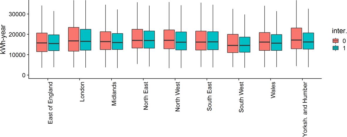
Figure 2. Average gas consumption by region compared by intervention group (0: no intervention, 1: any intervention)

The results of the model estimation for each region are summarized in Table 3. The average calculated r-squared is 0.82.

Table 3. Model estimation results by region

α δ β1 (WI) β2 (LI) β3 (B) ρ (temp) R2

all	1,320 (*)	0.88 (*)	-1,094 (*)	-390 (*)	-1,123 (*)	-301 (*)	0.82
East of England	1,221 (*)	0.89 (*)	-1,208 (*)	-256 (o)	-1,086 (*)	-333 (*)	0.83
London	1,299 (*)	0.89 (*)	-1,148 (*)	-234 (o)	-1,139 (*)	-373 (*)	0.83
Midlands	1,463 (*)	0.87 (*)	-1,128 (*)	-379 (*)	-1,060 (*)	-222 (*)	0.81
North East	1,515 (*)	0.87 (*)	-1,076 (*)	-403 (*)	-1,250 (*)	-330 (*)	0.79
North West	1,296 (*)	0.88 (*)	-1,017 (*)	-426 (*)	-1,088 (*)	-341 (*)	0.81
South East	1,255 (*)	0.89 (*)	-1,112 (*)	-441 (*)	-1,167 (*)	-327 (*)	0.83
South West	1,283 (*)	0.87 (*)	-869 (*)	-463 (*)	-1,177 (*)	-360 (*)	0.82
Wales	1,345 (*)	0.87 (*)	-835 (*)	-220 (o)	-1,359 (*)	-257 (*)	0.80
Yorksh. and Humber	1,394 (*)	0.88 (*)	-1,191 (*)	-429 (*)	-1,039 (*)	-207 (*)	0.81

(*): coefficient significant at a 95% confidence level, (o): coefficient not significant at a 95% confidence level

Firstly, Coursework代写

from the estimation of ρ, it can be concluded that the region most sensible to changes in temperature is London. In London a 1 degree Celsius increase in temperature results on average in savings of 373 kWh-year in gas consumption.

Regarding the intervention effect, wall insulation proves to be more effective in the East of England with average savings of 1,209 kWh-year. In the other hand, loft insulation is more effective in the South West, saving 463 kWh-year on average. Finally boiler replacement is more effective energy efficiency intervention overall, saving 1,359 kWh-year in Wales.

The loft insulation coefficient was not significant at a 95% confidence in Wales, East of England and London. This can be explained by the small effect that this intervention has in this regions.

Results by property type Coursework代写

To analyse the effect of building technique in the intervention effectiveness Figure 3 presents the average gas consumption by property type comparing between households with interventions and without. As expected, the largest average consumption is found in the detached houses (22,137 kWh-year), while the lowest is present in flats (11,157 kWh-year).

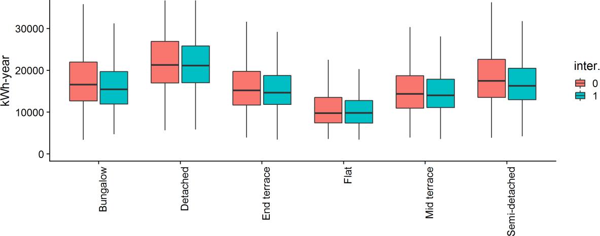
Figure 3. Average gas consumption by property type compared by intervention group (0: no intervention, 1: any intervention)

The results of the model estimation for each region are summarized in Table 4. The average calculated r-squared is 0.80.

Table 4. Model estimation results by property type

	α	δ	β1 (WI)	β2 (LI)	β3 (B)	ρ (temp)	R2
all	1,320 (*)	0.88 (*)	-1,094 (*)	-390 (*)	-1,123 (*)	-301 (*)	0.82
Bungalow	1,379 (*)	0.87 (*)	-600 (*)	-582 (*)	-1,204 (*)	-263 (*)	0.81
Detached	1,894 (*)	0.88 (*)	-1,654 (*)	-651 (*)	-1,049 (*)	-435 (*)	0.80
End terrace	1,524 (*)	0.86 (*)	-1,217 (*)	-363 (*)	-1,063 (*)	-226 (*)	0.79
Flat	1,040 (*)	0.86 (*)	-654 (*)	-613 (*)	-1,097 (*)	-144 (*)	0.81
Mid terrace	1,671 (*)	0.84 (*)	-1,016 (*)	-275 (*)	-943 (*)	-228 (*)	0.76
Semi detached	1,588 (*)	0.87 (*)	-1,175 (*)	-311 (*)	-1,231 (*)	-337 (*)	0.80

(*): coefficient significant at a 95% confidence level, (o): coefficient not significant at a 95% confidence level

Wall insulation proves to be more effective in detached dwellings with average savings of 1,654 kWh-year, same for loft insulation with average saving 651 kWh- year on average. Finally boiler replacement is more effective in semidetached dwellings, saving 1,231 kWh-year. Regarding temperature sensibility, it can be concluded that property type most sensible to weather changes is detached dwelling with an average impact 435kWh for each 1 degree Celsius decrease in average temperature.Coursework代写

Even though all the coefficients estimates are significant is important to review the significance of loft insulation in flats. As exposed in Table 1, 103 loft insulation where done in flats (corresponding to top floor flats) which is not a large sample compared to the control group.

By property age

Figure 4 presents the average gas consumption by each property age range, comparing between households with interventions and without. The largest average consumption is found in the houses built between 1930 and 1949 (18,900 kWh-year),while the lowest is present in the houses built between 1983 and 1995 (15,598 kWh- year).Coursework代写

Figure 4. Average gas consumption by property age compared by intervention group (0: no intervention, 1: any intervention)

The results of the model estimation for each property age band are summarized in Table 5. The average calculated r-squared is 0.83.

Table 5. Model estimation results by property age

	α		δ		β1 (WI)	β2 (LI)	β3 (B)	ρ (temp)	R2
all		1,320 (*)		0.88 (*)	-1,094 (*)	-390 (*)	-1,123 (*)	-301 (*)	0.82
Before 1930		900 (*)		0.91 (*)	-911 (*)	-138 (o)	-639 (*)	-214 (*)	0.85
1930 to 1949		1,572 (*)		0.87 (*)	-1,149 (*)	-347 (*)	-1,285 (*)	-373 (*)	0.80
1950 to 1966		1,377 (*)		0.87 (*)	-1,082 (*)	-402 (*)	-1,229 (*)	-292 (*)	0.80
1967 to 1982		1,283 (*)		0.88 (*)	-975 (*)	-507 (*)	-1,225 (*)	-235 (*)	0.82
1983 to 1995		907 (*)		0.9 (*)	-1,014 (*)	-386 (*)	-930 (*)	-310 (*)	0.87
1996 onwards		900 (*)		0.91 (*)	-911 (*)	-138 (o)	-639 (*)	-214 (*)	0.85

(*): coefficient significant at a 95% confidence level, (o): coefficient not significant at a 95% confidence level

Wall insulation proves to be more effective in dwellings built between 1930 and 1949 with average savings of 1,149 kWh-year. With loft insulation the most effective group is dwellings built between 1967 and 1982 with average saving of 651 kWh-year. Finally boiler replacement is more effective in dwellings built between 1930 and 1949, saving 1,229 kWh-year on average. With this results is important to highlight that the effects of interventions are more significant in older dwellings, as expected. Dwellings built between 1930 and 1949 are the most sensible to temperature.

The model coefficient for loft insulation in dwellings built before 1930, and after 1996 is statistically non-significant at a 95% confidence level. This can be explained by the small average affect that these interventions have in this dwellings.

By floor size Coursework代写

Finally, in order to exclude the effects of larger consumption due to larger heating space form the results, is relevant to conduct the analysis by property size. Figure 5

presents the average gas consumption by property size band comparing between households with interventions and without. As expected, the largest average consumption is found in dwellings with floor area larger than 151 sqm (26,614 kWh- year), while the lowest is present in the smallest dwellings (10,362 kWh-year).

Figure 5. Average gas consumption by property size compared by intervention group (0: no intervention, 1: any intervention)

The results of the model estimation for each region are summarized in Table 6. The average calculated r-squared is 0.78.Coursework代写

Table 6. Model estimation results by property size

	α		δ		β1 (WI)	β2 (LI)	β3 (B)	ρ (temp)	R2
all		1,320 (*)		0.88 (*)	-1,094 (*)	-390 (*)	-1,123 (*)	-301 (*)	0.82
1 to 50		821 (*)		0.87 (*)	-550 (o)	-227 (o)	-1,089 (*)	-113 (*)	0.82
51 to 100		1,712 (*)		0.84 (*)	-801 (*)	-290 (*)	-1,060 (*)	-229 (*)	0.76
101 to 150		2,234 (*)		0.85 (*)	-1,450 (*)	-631 (*)	-1,225 (*)	-375 (*)	0.76
Over 151		2,814 (*)		0.86 (*)	-1,413 (*)	-390 (o)	-776 (*)	-548 (*)	0.76

(*): coefficient significant at a 95% confidence level, (o): coefficient not significant at a 95% confidence level

All of three interventions analyzed prove to be more effective in dwellings with floor area between 101 and 150 sqm, saving 1,450 kWh-year, 631 kWh-year, 1,225 kWh- year for wall insulation, loft insulation and boiler replacement respectively. Regarding temperature sensibility, it can be concluded that large dwellings are the most sensible to weather changes with an average impact 548 kWh-year per 1 degree Celsius decrease in average temperature.Coursework代写

Similar to previous groups, due to the small average effect, loft insulation effect is non-significant in dwellings up to 50 sqm and larger than 151sqm.

5. Discussion and conclusions

Heat decarbonization remains a big challenge for the UK’s energy system. While the technological low carbon alternatives for gas are under development, the large

potential in the application of energy efficiency measures for reducing heat demand, highlights the relevance to prioritize energy efficiency interventions when addressing heat decarbonization and fuel poverty. Therefore, from a public policy perspective is relevant to quantify the effects of energy efficiency measures, while distinguishing policy between the spatial characteristics of the dwelling.

To summarize the results of this analysis,Coursework代写

Table 7 presents the impact of energy efficiency interventions relative to the average consumption by each group of dwellings. This table can be relevant input for policy makers when addressing energy efficiency programs.

Table 7. Energy efficiency intervention impact relative to 2012 gas consumption.

Gas cons. WI LI B Gas cons. WI LI B

  all 14,588    -7.5%   -2.7%   -7.7%  all 14,588 -7.5% -2.7% -7.7% 

East of Eng.	14,308	-8.4%		-7.6%		Bungalow	14,163	-4.2%	-4.1%	-8.5%
London	15,495	-7.4%		-7.3%		Detached	19,312	-8.6%	-3.4%	-5.4%
Midlands	14,492	-7.8%	-2.6%	-7.3%		End terrace	13,489	-9.0%	-2.7%	-7.9%
North East	14,961	-7.2%	-2.7%	-8.4%		Flat	9,271	-7.1%	-6.6%	-11.8%
North West	14,533	-7.0%	-2.9%	-7.5%		Mid terrace	12,613	-8.1%	-2.2%	-7.5%
South East	15,028	-7.4%	-2.9%	-7.8%		Semi-det.	15,000	-7.8%	-2.1%	-8.2%
South West	13,211	-6.6%	-3.5%	-8.9%
Wales	13,577	-6.2%		-10.0%
Yorksh. & Hum.	14,867	-8.0%	-2.9%	-7.0%

Gas cons. WI LI B Gas cons. WI LI B Coursework代写

  all 14,588    -7.5%   -2.7%   -7.7%  all 14,588 -7.5% -2.7% -7.7% 

bef. 1930	15,873	-5.7%		-4.0%		1 to 50	8,589			-12.7%
1930-1949	15,989	-7.2%	-2.2%	-8.0%		101-150	17,548	-4.6%	-1.7%	-6.0%
1950-1966	13,744	-7.9%	-2.9%	-8.9%		51-100	12,140	-11.9%	-5.2%	-10.1%
1967-1982	13,516	-7.2%	-3.8%	-9.1%		Over 151	23,733	-6.0%		-3.3%
1983-1995	13,485	-7.5%	-2.9%	-6.9%
1996 onw.	14,066	-6.5%		-4.5%

Non-siginificant estimates at a 95% confidence level are excluded from the results.

It is concluded that wall insulation is more effective on end terrace dwellings on the East of England, built between 1950 and 1966 with a floor size between 51 and100 sqm, saving on average 9.3% on gas consumption. Loft insulation has the largest impact on bungalows on the Southwest built between 1967 and 1982 with a floor area between 51 and 100 sqm, saving on average 4.1% on gas consumption. Finally, boiler replacement is the most effective when applied to flats in Wales built between 1967 and 1982 with a floor area smaller than 50sqm, saving on average 10.9% on gas consumption.Coursework代写

In order to make this analysis a starting point for research is imporantat to highlight the main limitations of the analysis and address key points for future work:

• Each model considered subsets by one dwelling characteristics at the time, therefore the sample within the group is not necessarilycomparable regarding the other dwelling
• The compound effect of multiple interventions done in the same dwelling is not consider. This is captured in the model as the linear sum of coefficients which differs from reality.
• As future work, it is interesting to conduct a cost benefit analysis of each intervention by type of household and by floor area, in order to find the most cost effective

6. Bibliography Coursework代写

Adan, H. and Fuerst, F. (2016) ‘Do energy efficiency measures really reduce household energy consumption? A difference-in-difference analysis’, Energy Efficiency. Energy Efficiency, 9(5), pp. 1207–1219. doi: 10.1007/s12053-015-9418- 3.

Aksözen, M. et al. (2015) ‘Building age as an indicator for energy consumption’,

Energy and Buildings, 87, pp. 74–86. doi: 10.1016/j.enbuild.2014.10.074.

Anderson, J. E., Wulfhorst, G. and Lang, W. (2015) ‘Energy analysis of the built environment – A review and outlook’, Renewable and Sustainable Energy Reviews. Elsevier, 44, pp. 149–158. doi: 10.1016/j.rser.2014.12.027.

Asadi, E. et al. (2014) ‘Multi-objective optimization for building retrofit: A model using genetic algorithm and artificial neural network and an application’, Energy and Buildings, 81, pp. 444–456. doi: 10.1016/j.enbuild.2014.06.009.

Battista, G. et al. (2014) ‘Buildings energy efficiency: Interventions analysis under a smart cities approach’, Sustainability (Switzerland), 6(8), pp. 4694–4705. doi: 10.1016/j.apenergy.2017.07.087.

Braun, F. G. (2010) ‘Determinants of households’ space heating type: A discrete choice analysis for German households’, Energy Policy. Elsevier, 38(10), pp.

5493–5503. doi: 10.1016/j.enpol.2010.04.002.

Van Den Brom, P., Meijer, A. and Visscher, H. (2018) ‘Performance gaps in energy consumption: household groups and building characteristics’, Building Research and Information. Taylor & Francis, 46(1), pp. 54–70. doi: 10.1080/09613218.2017.1312897.Coursework代写

Brounen, D., Kok, N. and Quigley, J. M. (2012) ‘Residential energy use and conservation: Economics and demographics’, European Economic Review. Elsevier, 56(5), pp. 931–945. doi: 10.1016/j.euroecorev.2012.02.007.

Croissant, Y. and Millo, G. (2008) ‘Panel Data Econometrics in R : The plm Package’, Journal of Statistical Software, 27(2). doi: 10.18637/jss.v027.i02.

Crosbie, T. and Baker, K. (2010) ‘Energy-efficiency interventions in housing: Learning from the inhabitants’, Building Research and Information, 38(1), pp. 70– 79. doi: 10.1080/09613210903279326.Coursework代写

Dall’O’, G., Galante, A. and Pasetti, G. (2012) ‘A methodology for evaluating the potential energy savings of retrofitting residential building stocks’, Sustainable

Cities and Society. Elsevier B.V., 4(1), pp. 12–21. doi: 10.1016/j.scs.2012.01.004.

Doukas, H., Nychtis, C. and Psarras, J. (2009) ‘Assessing energy-saving measures in buildings through an intelligent decision support model’, Building and Environment, 44(2), pp. 290–298. doi: 10.1016/j.buildenv.2008.03.006.

Fowlie, M., Greenstone, M. and Wolfram, C. (2018) ‘Do Energy Efficiency

Investments Deliver? Evidence from the Weatherization Assistance Program’, The Quarterly Journal of Economics, 133(3), pp. 1597–1644.

Frederiks, E. R., Stenner, K. and Hobman, E. V. (2015) ‘The socio-demographic and psychological predictors of residential energy consumption: A comprehensive review’, Energies, 8(1), pp. 573–609. doi: 10.3390/en8010573.

Gillingham, K., Newell, R. G. and Palmer, K. (2010) ‘Energy efficiency: Economics and policy’, Journal of Economic Surveys, 24(3), pp. 573–592. doi: 10.1111/j.1467- 6419.2009.00609.x.Coursework代写

Guerra-Santin, O. and Itard, L. (2010) ‘Occupants’ behaviour: Determinants and effects on residential heating consumption’, Building Research and Information, 38(3), pp. 318–338. doi: 10.1080/09613211003661074.

Haines, A. et al. (2009) ‘Public health benefits of strategies to reduce greenhouse- gas emissions: household energy’, The Lancet, 374(9705), pp. 1917–1929. doi: 10.1016/S0140-6736(09)61713-X.

Hamilton, I. G. et al. (2013) ‘Energy epidemiology: A new approach to end-use energy demand research’, Building Research and Information, 41(4), pp. 482–497. doi: 10.1080/09613218.2013.798142.

Hamilton, I. G. et al. (2014) ‘Uptake of energy efficiency interventions in English dwellings’, Building Research and Information. Taylor & Francis, 42(3), pp. 255– 275. doi: 10.1080/09613218.2014.867643.

Heinonen, J., Kyrö, R. and Junnila,

S. (2011) ‘Dense downtown living more carbon intense due to higher consumption: A case study of Helsinki’, Environmental Research Letters, 6(3). doi: 10.1088/1748-9326/6/3/034034.

Heo, Y., Choudhary, R. and Augenbroe, G. A. (2012) ‘Calibration of building energy models for retrofit analysis under uncertainty’, Energy and Buildings, 47, pp. 550–560. doi: 10.1016/j.enbuild.2011.12.029.

Huebner, G. M. et al. (2015) ‘Explaining domestic energy consumption – The comparative contribution of building factors, socio-demographics, behaviours and attitudes’, Applied Energy, 159, pp. 589–600. doi: 10.1016/j.apenergy.2015.09.028.

Jackson, T. and Druckman, A. (2008) ‘Household energy consumption in the UK: A highly geographically and socio-economically disaggregated model’, Energy Policy, 36(8), pp. 3167–3183.Coursework代写

Lee, C. C. (2005) ‘Energy consumption and GDP in developing countries: A cointegrated panel analysis’, Energy Economics, 27(3), pp. 415–427. doi:

10.1016/j.eneco.2005.03.003.

Ofgem (2016) The Decarbonisation of Heat (Ofgem’s Future Insights Series), Ofgem ’ s Future Insights Series.

Pelenur, M. J. and Cruickshank, H. J. (2012) ‘Closing the Energy Efficiency Gap: A study linking demographics with barriers to adopting energy efficiency measures in the home’, Energy, 47(1), pp. 348–357. doi: 10.1016/j.energy.2012.09.058.

Scott, F. L., Jones, C. R. and Webb, T. L. (2014) ‘What do people living in deprived communities in the UK think about household energy efficiency interventionsα’, Energy Policy, 66, pp. 335–349. doi: 10.1016/j.enpol.2013.10.084.

Steemers, K. and Ben, H. (2014) ‘Energy retrofit and occupant behaviour in protected housing: A case study of the Brunswick Centre in London’, Energy and Buildings, 80, pp. 120–130.

UK BEIS (2018) 2017 UK Greenhouse Gas Emissions, Provisional Figures: Statistical release.Coursework代写

Wang, S. S. et al. (2011) ‘CO2 emissions, energy consumption and economic growth in China: A panel data analysis’, Energy Policy, 39(9), pp. 4870–4875. doi: 10.1016/j.enpol.2011.06.032.Coursework代写

Wooldrige, Jeffrey, M. (2011) ‘Econometric Analysis of Cross Section and Panel Data’, Neurology Secrets, 7, pp. i–ii. doi: 10.1515/humr.2003.021.

Zhou, K. and Yang, S. (2016) ‘Understanding household energy consumption behavior: The contribution of energy big data analytics’, Renewable and Sustainable Energy Reviews, 56, pp. 810–819. doi: 10.1016/j.rser.2015.12.001.

更多其他：C++代写 r代写  考试助攻 C语言代写 finance代写 lab代写 计算机代写 code代写 report代写 project代写 物理代写 数学代写 java作业代写 经济代写  course代写

合作平台：天才代写 幽灵代写 写手招聘 Essay代写