
Identification of Auction Models Using Order Statistics
Order Statistics代写 Auction data often fail to record all bids or all relevant factors that shift bidder values. In this paper,
Yao Luo∗ Ruli Xiao† March 1, 2019
Abstract Order Statistics代写
Auction data often fail to record all bids or all relevant factors that shift bidder values. In this paper, we study the identification of auction models with unobserved heterogeneity (UH) using multiple order statistics of bids. Classical measurement error approaches require multiple independent measurements.
Order statistics, by definition, are dependent, rendering classical approaches inapplicable. First, we show that models with nonseparable finite UH is identifiable using three consecutive order statistics or two consecutive ones with an instrument. Second, two arbitrary order statistics identify the models if UH provides support variations. Third, models with separable continuous UH are identifiable using two consecutive order statistics under a weak restrictive stochastic dominance condition. Lastly, we apply our meth- ods to U.S. Forest Service timber auctions and find evidence of UH.
JEL: C14, D44
Key Words: Unobserved Heterogeneity, Measurement Error, Finite Mixture, Multi- plicative Separability, Support Variations, Deconvolution
∗Department of Economics, University of Toronto, Max Gluskin House, 150 St. George St, Toronto,ON M5S 3G7. Email: yao.luo@utoronto.ca.
†Department of Economics, Indiana University, 100 S. Woodlawn Ave. Bloomington, IN 47405.
Email: rulixiao@iu.edu.
1 Introduction Order Statistics代写
Recent years have seen a growth of the literature combing auction theory with economet- ric analysis to understand auctions markets and inform policy. While the key elements in auction theory normally match well the practice, it is less so when there is auction-level heterogeneity. Not only auctions differ in observable characteristics, there are factors affecting bidder values that are common knowledge among bidders but unobserved by the analyst. Ignoring such factors, known as unobserved heterogeneity(UH), leads to erroneous estimates and wrong policy conclusions.
The earliest approach
to allow for UH in auctions exploits an auxiliary variable that is monotone in UH. See, e.g., Campo, Perrigne, and Vuong (2003) and Haile, Hong, and Shum (2003). Later there are two streams of measurement error approaches that exploit multiplicity of bids in each auction to deal with discrete and continuous UH, respectively. A common feature of these approaches is that they all require multiple measurements, which are independent conditioning on UH. Bids, however, are missing non-randomly for all kinds of reasons. Specifically, we may observe multiple order statistics of all the bids rather than all or multiple independent bids.
For instance, Kim and Lee (2014) observe
the second to the fourth highest bids in ascending used-car auctions. U.S. Forest Service timber auctions only record at most the top 12 bids regardless the number of bidders. Freyberger and Larsen (2017) observe the second and third order statistics of bids in eBay auctions for used iPhones. Naturally, these order statistics are dependent, leading to failure in identification following the usual measurement error approaches. This paper shows that despite of being dependent, the same number of order statistics as that of the independent measurements are sufficient to achieve similar identification results for auctions with discrete or continuous UH.
Our first result shows that three consecutive order statistics of bids,Order Statistics代写
despite of theirdependence, identifies independent private value (IPV) auction models with nonsepara-ble finite UH. In usual misclassification models, independence among multiple measure- ments implies that the joint distribution have a multiplicatively separable structure with which eigen-decomposition of the matrix constructed by the joint distribution of observed measurements pins down the type-specific distribution as the eigenvalue/eigenvector ma- trix with a full rank condition.
The same multiplicative separable structure Order Statistics代写
does not exist in the scenario with order statistics because of the dependence by its nature. The joint distribution of consecutive order statistics, however, can be constructed to a sim- ilar separable structure. This separability is mainly induced by the consecutive feature of the order statistics. Consequently, we can identify the auction models using simi- lar eigen-decomposition with a suitable rank condition. Similar identification argument can be extended to the scenario of only two consecutive order statistics with a binary instrumental variable.
Our second result shows that the auction models with finite
UH can be identified using any two order statistics of bids with strict support variations. This result extends Hu and Sasaki (2017), which identify the model with nonseparable finite UH exploiting monotonicity of support boundaries in UH with two independent measurements. It is also related to D’Haultfœuille and F´evrier (2015) which identify nonseparable measure- ment error models using support variations and three measurements. While they exploit the joint distribution of the measurements being multiplicatively separable, we can not do the same with order statistics.
Support variations lead to density discontinuities at the upper boundaries of com- ponent distributions.
These discontinuity points divide bid support into intervals, and order statistics from lower type distributions have positive densities only in lower inter- vals. Identification then follows from an induction argument. First, the highest type solely determines the conditional distribution of the lower order statistic conditioning on the larger one being in the most upper interval. As a result, we can back out the distribution of the highest type.Order Statistics代写
Second, we can subtract the contribution of the highest type from the same conditional distribution in the second most upper interval to obtain the contribution of the second highest type and then identify its distribution. Iterating this argument identifies all component distributions. Lastly, we extend these results for first price auctions to allow for multiple sources of UH: unobserved competition and unobserved auction type. Identification requires an ordering condition which can be satisfied with first oder stochastic dominance ordering type-specific value distribution.
Our last result concerns identification of auctions with continuous UH.
Following the existing literature, we assume UH is additively separable in bidder value, which consti- tutes an error-in-variable model.
While identification with multiple independent mea- surements is well-known for this model (Li and Vuong (1998), Li, Perrigne, and Vuong (2000), and Krasnokutskaya (2011)), the same problem with multiple order statistics is unsolved (Athey and Haile (2002)). Specifically, the dependence among order statistics precludes applications of the classical approach, which relies on both the “within” inde- pendence between value and UH, and the “between” independence of values. However, the latter no longer applies to order statistics.
Instead, we propose a new identification strategy that relies only on the “within” independence.
Moreover, it exploits properties of consecutive order statistics. In par- ticular, we show that any two consecutive order statistics are sufficient to identify the model in two steps. First, we show that the top two order statistics are sufficient for identification.
The “within” independence identifies the ratio of the characteristic func- tions of top two order statistics. This ratio determines the parent distribution under a weak assumption. This result extends to the case with a maximum order statistic and any other order statistic. Second, any two consecutive order statistics identify the distributions of a maximum order statistics and a minimum order statistic, which again achieves identification following similar arguments in the first step.Order Statistics代写
Literature Review
For discrete UH with nonseparable structure by nature, the existing literature uses the eigen-decomposition approach, as in Hu, McAdams, and Shum (2013). They achieve identification using bid information of at least three bidders per auction following the results of Hu (2008).
Recently,
Hu and Sasaki (2017) show that two independent proxies of the latent factor are sufficient to identify nonseparable measurement error model if the support boundaries are increasing with respect to UH, which can also be applied to auction models. For continuous UH, the existing literature uses the deconvolution ap- proach, as in Li and Vuong (1998), Li, Perrigne, and Vuong (2000), and Krasnokutskaya (2011), among others. They require two random bids in each auction and restrict that the UH has a separable structure on bidders’ values.
There have been increasing interest in using order statistics for identification in theauction literature. Many markets can be treated as auctions where only the transaction price is observed. Athey and Haile (2002) show that the auction model with symmetric independent private values (IPV) is identified with the transaction price and the number of bidders.
This exploits a one-to-one mapping between a parent distribution
and the distribution of an order statistic. Guerre and Luo (2018) show that the auction model with symmetric IPV and unknown competition is identified using the transaction price only. They exploit discontinuities in the density function of the winning bid due to changing competition.
Some data contain multiple order statistics of bids.
Song (2004) considers eBay auctions where the number of bidders is random and unobservable. He shows that any two order statistics identifies the symmetric IPV model. Freyberger and Larsen (2017) study eBay auctions for used iPhones with auction-specific unobserved heterogeneity and an unknown number of bidders. They circumvents the issue of correlated order statistics using observed reserve prices, rendering the identification problem classical. Kim and Lee (2014) apply the identification results of Song (2004) to wholesale used-carauctions in Korea. Due to the ascending auction format, they observe the second, third and fourth highest bids but not the first highest bids.
Related to our first result,
Mbakop (2017) takes a different approach that tries to restore the conditional independence structure needed in the usual approaches. In par- ticular, he exploits the Markov property of order statistics and shows that the bidder’s UH-specific distribution and the distribution of UH is point identified from either (any) five or three order statistics along with an instrument using the joint distribution of three order statistics conditional on the two middle order statistics. In contrast, we take advantage of the separability structure provided by consecutive order statistics and achieve identification using three consecutive order statistics. Moreover, our results also extends to (any) four order statistics.
This paper is organized as follows. In Section 2 we describe the auction models. Section 3 and 4 presents identification results of nonseparable finite UH and separable continuous UH, respectively. Section 5 presents an application of the identification result into USFS timber auctions. Section 6 concludes.
2 IPV Auction Models with UH
In this section, we introduce standard IPV auction with UH. Suppose n ≥ 2 symmetric bidders participate in an auction with zero reserve price. Bidders are risk neutral. Conditioning on an auction-level UH k, where k can be discrete finite or continuous, bidders’ valuations are i.i.d. draws from the same distribution Φk(v) with support [v, vk]. All bidders simultaneously submit bids. We denote the optimal bid distribution for the auction state k as F k(x), and the optimal bid x is with support [x, xk].
2.1 The first-price auction model
In a first-price auction, the bidder with the highest bid wins and pays the price he/she submitted. In a state-k auction, a bidder with a valuation v chooses his bid b to maximize its expected payoff, represented in the following.
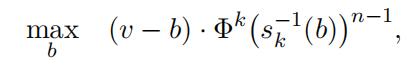
where s−1(·) is the inverse of his/her optimal bidding strategy in state-k auctions, and Φk(s−1(b))I−1 is the chance of winning.
Guerre, Perrigne, and Vuong (2000) study the identification of the type-specific value distribution Φk(·) when the competition level n and the type-specific bid distributionF k(·) is observed. In particular, the identification comes from the type-specific one-to-one mapping between the unknown value and the observed type-specific bid distribution function:
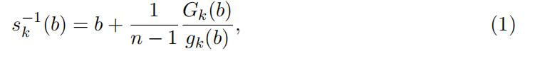
where b is any arbitrary bid in its support, and ttk(·) and gk(·) are the type-specific bid distribution and density functions, respectively.
2.2 The second-price auction model
In a second-price auction, the bidder with the highest bid wins and pays the second high- est price submitted. In the private value framework, second-price auctions are equivalent to ascending auctions. Optimal bidding behaviors in these auctions are straightforward: a weakly dominant strategy is to stay in the bidding until the standing bid reaches your value. In other words, once the next-to-last bidder drops out, the bidder with the highest value wins at a price equal to the second-highest value. Therefore, the highest bid is never observed. Moreover, the observed bids are the rth order statistics from an auction of number of bidders n from the value distributions Φk(·), where r ≤ n − 1.
If the number of bidders n and the distribution for the winning bid,
which is thedistribution of the n−1th order statistics out of a n ordered sample denoted as F k (·),is known, the unknown type-specific bid function F k(·) can be identified because there is a one-to-one mapping between the distribution of the (n − 1)th order statistics and the underlying distribution itself. That is,
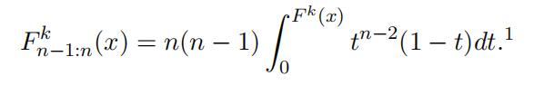
Once we recover the type-specific bid distribution from the distribution of the type- specific order statistics, we identify the type-specific value distribution as
Φk(x) = F k(x). (2)
In summary,
we can identify the type-specific value distributions Φk(·) from the type-specific bid distributions F k(·) for the first price auction using equation (1) and for the second price auction using equation (2). Consequently, we focus on identification of the type-specific bid distribution F k(·) from the joint distribution of order statistics of the bids. We then can follow the above argument to recover the type-specific value distribution.
1In general, the distribution function of the rth order statistic Xr:n is
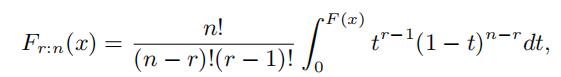
which is strictly increasing in F (x) and thus invertable. Therefore, the distribution of any order statistic identifies the parent distribution F (x). This property has been used in several papers including Athey and Haile (2002) and Song (2004).
3 Identification with Nonseparable UH
In this section, we consider the generic identification of nonseparable UH in auction models. First, we derive some properties of order statistics which is essential for our identification. Then we provide sufficient conditions to identify the type-specific bid distributions using three consecutive order statistics. We then extend the identifica- tion result to the case with two consecutive order statistics and an instrument variable. Second, we provide identification using only two consecutive order statistics with a first order stochastic dominance condition (FOSD). This result can be extended to the scenar- ios of multi-dimensional UH such as allowing for the number of bidders to be unknown for first price auction.
We first introduce some notation.
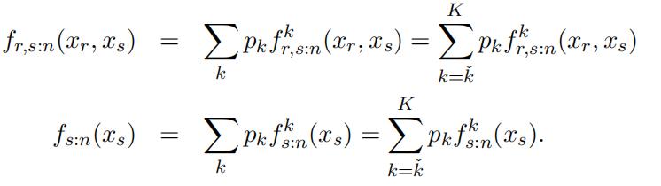
There are K unobserved value types, assumed to be finite and discrete, which maps to K unobserved bid distributions. We assume that the cardinality of the UH K is known.2 The probability of type k is pk, so k pk = 1.Let X1:n ≤ X2:n ≤, …, ≤ Xn:n represent the n order statistics out of an n ordered sample,and x1 ,…, xn represent their realizations, respectively. We use fr,s,j:n(·) to denote thejoint pdf of the three order statistics Xr:n, Xs:n, Xj:n, we use fr|s:n(·, ·) to denote theconditional pdf of order statistics Xr:n|Xs:n, and we use fr:n(·) to denote the marginal distribution of order statistics Xr:n. The cdfs F (·) are defined analogously.
3.1 PreliminariesOrder Statistics代写
We now derive two useful properties of order statistics that we exploits in our identi- fication arguments. We first illustrate that the joint distribution of consecutive order statistics persists the multiplicatively separable structure in a restricted region by the definition of order statistics. We then illustrate how the conditional distribution of or- der statistics determines the distribution of another order statistic, which leads to the identification of the parent distribution. We omit UH in this subsection.
2When K is unknown, some rank condition would be sufficient to identify the cardinality of the unobserved types K as in An (2017)
Separability by consecutiveness
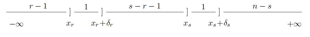
Suppose we observe two order statistics out of an n ordered sample, Xr:n, Xs:n, where r < s. To understand the separability generated by two consecutive order statistics, we visualize the event (xr < Xr:n ≤ xr+δr, xs < Xs:n ≤ xs+δs) with xr+δr ≤ xs in Figure 1. When δr and δs are both small, the likelihood of this event is approximately proportional to the multiplication of the following three components: (1) the probability that r − 1 draws are smaller than xr, F (xr)r−1; (2) the probability that 1 draw is in (xr, xr + δr),
f (xr)δr; (3) the probability that n − s draws are larger than xs, [1 − F (xs)]n−s; (4) the probability that 1 draw is in (xs, xs + δs), f (xs)δs; (5) the probability that s − r − 1 draws are in between xr + δr and xs, [F (xs) − F (xr)]s−r−1. Thus, the likelihood of this event can be represented in a multiplicatively separable structure in xr and xs if and only if s − r − 1 = 0, i.e., the two order statistics are consecutive.Order Statistics代写
Figure 1: Joint Distribution of Two Consecutive Order Statistics
Similar logic can be applied to the joint distribution of three order statistics. Sup- pose we observe three consecutive order statistics, Xr−2:n, Xr−1:n, Xr:n. The well-known Markovian property of order statistics implies that
fr−2,r−1,r:n(xr−2, xr−1, xr) = fr−1:n(xr−1)fr−2|r−1:n(xr−2|xr−1)fr|r−1:n(xr|xr−1). (3)
The two conditional density functions of two consecutive order statistics fr−2|r−1:n(xr−2|xr−1) and fr|r−1:n(xr|xr−1) are multiplicatively separable because their joint density functions are multiplicatively separable.
Furthermore, we can represent the above joint distribu-tion as the following multiplicatively separable structure:
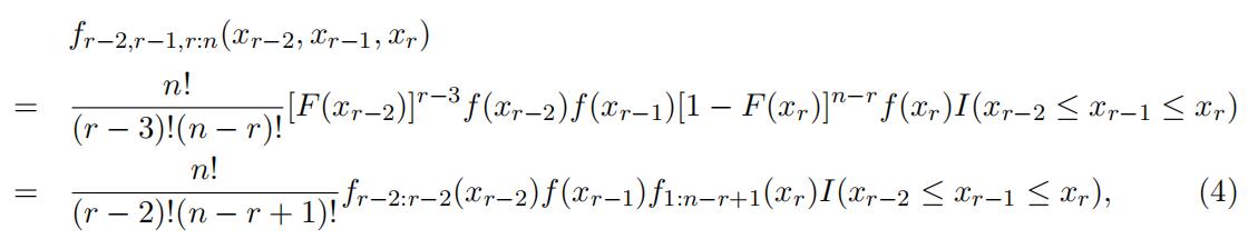
where I(·) is the indicator function. Intuitively, we can visualize the event (xr−2 < Xr−2:n ≤ xr−2 + δr−2, xr−1 < Xr−1:n ≤ xr−1 + δr−1, xr < Xr:n ≤ xr + δr) in Fig-
ure 2. The likelihood of this event is proportional to the multiplication of the fol- lowing three components: (1) the probability that one draw is in (xr−1, xr−1 + δr−1),
f (xr−1)δr−1; (2) the probability that the maximum of r − 2 draws are in (xr−2, xr−2 +
δr−2), fr−2:r−2(xr−2)δr−2; (3) the probability that the minimum of n − r + 1 draws are in (xr, xr + δr), f1:n−r+1(xr)δr.Order Statistics代写
Figure 2: Joint Distribution of Three Consecutive Order Statistics
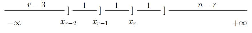
Even though order statistics are correlated by their nature, the joint distribution of three consecutive order statistics can be separated as the products of three marginaldistributions fr−2:r−2(xr−2), f (xr−1),
and f1:n−r+1(xr) in the area of xr−2 ≤ xx−1 ≤xr.Note that this separability does not indicate that the three order statistics areindependent. The separability only holds in the region xr−2 ≤ xx−1 ≤ xr, but not for the full support [x, x¯] × [x, x¯] × [x, x¯]. The joint probability distribution is zero outside the region xr−2 ≤ xx−1 ≤ xr. This is due to the definition of the order statistics, i.e., Xr−2:n ≤ Xx−1:n ≤ Xr:n.
Conditional Distribution of Order Statistics Order Statistics代写
Consider again any two order statistics Xr:n and Xs:n, where r < s. The conditional density of Xr:n given that Xs:n = xs can be written as
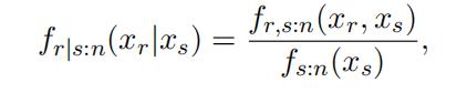
Figure 1 visualizes the event
(xr < Xr:n ≤ xr + δr, xs < Xs:n ≤ xs + δs) and the event (xs < Xs:n ≤ xs + δs). While the likelihood of the former is proportional to f (xr)f (xs)·F (xr)r−1 ·[1−F (xs)]n−s ·[F (xs)−F (xr)]s−r−1 as shown above, the likelihood of the latter is proportional to the multiplication of: (1) the probability that s − 1 draws are smaller than xs, F (xs)s−1; (2) the probability that 1 draw is in (xs, xs + δs), f (xs)δs;theprobability that n − s draws are larger than xs, [1 − F (xs)]n−s.
Therefore, the ratio that defines the conditional density is proportional to f(xr )
In fact, it is the same as the distribution of the rth order statistic in a sample of size s − 1 from a distribution that is the parent distribution truncated at xs. Note that the truncation is no longer effective if xs = x. As a result,the conditional distribution is the same as the distribution of the rth order statistic in a sample of size s − 1 from the parent distribution F (·).
3.2 Identification using three consecutive order statistics
This subsection uses the separability properties of consecutive order statistics in a certain region to provide sufficient condition to identify auction models with nonseparable UH with a known competition level. The identification proceeds in several steps.
First,
we apply a discretization to the bid support which accounts for the ordering of the observed order statistics so that the separable structure persists. Second, an eigenvalue decomposition argument identifies a key matrix that governs the finite mixture structure in our order statistic setting. Third, we apply this matrix to identify the componentdistributions in the lower portion of the support and then in the upper part.The unconditional joint distribution of any three consecutive order statistics, which can be estimated from the data directly, by total probability can be represented as
This joint distribution of the consecutive order statistics
has a semi-separable structure,in the sense that we can separate the observed joint density function into three den-sity functions, which is similar to that in the finite mixture literature, but it has an extra restriction by the nature of order statistics I(xr−2 ≤ xr−1 ≤ xr), which cannot be separated. This semi-separable structure precludes us from following exactly the identification procedure in the existing literature to identify the type-specific bid dis- tribution.
However,
the restriction by the indicator function can be safely ignored if we divide the original support by two cutoff points x < c1 < c2 < x¯ to separate the support into three parts, referred to as “low”, “middle”, and “high” and denoted as l ≡ [x, c1], m ≡ [c1, c2], and h ≡ [c2, x¯], respectively. The separable structure of the joint distribution fr−2,r−1,r:n(xr−2, xr−1, xr) reappears if we always restrict xr−2 ∈ l, xr−1 ∈ m, and xr ∈ h. Specifically, if xr−2 ∈ l, xr−1 ∈ m, and xr ∈ h, the joint distribution can be expressed as

which has a familiar structure of finite mixture models but each component has different meanings.
Following the existing literature,
we first select K exclusive intervals from the “low”support l and the “high” support h, denoted as li and hi, i = 1, …, K, respectively. We also select 2 exclusive intervals from the “middle” support m, denoted as mi, i = 1, 2. Note that these intervals do not have to be fully exhaustive, and they can be simply points. Figure 3 provides a visualization of the support.
Figure 3: Support Visualization

We then rewrite the above joint distribution with respect to the selection of the support:
Similar to the identification in finite mixture and measurement error literature, the identification uses matrix algebra, so we first define the following matrix notation.
where Jl,mij ,h denotes the joint probability matrix with the i,
jth element being the probability of the event {Xr−2:n ∈ li, Xr−1:n ∈ mij , Xr:n ∈ hj}; L is is the probability matrix for top order statistics Xr−2:r−2 with the i, kth element being the probability of the event {Xk ∈ li}, where i, k = 1, …, K; Dm is the diagonal matrix withijthe kth diagonal element being the probability of the event {X ∈ mij };Dp is the diagonal type weight matrix with the kth diagonal element being the weight of type k;
H is the probability matrix for the bottom statistics X1:n−r+1 with the i, kth elementbeing the probability of the event {Xk ∈ hi}. With the matrix notation, we havethe following matrix representation connecting the observed joint probability with the unknown matrix constructed using type-specific probability:

Following the existing literature, identification of models with UH using the mixture features usually requires some rank condition, which is stated in the follows.
Assumption 1.
(Full Rank) There exists a mapping from xr−2 and xr into K inter- vals of the support [x, x¯] so that the probability matrix in the “low” support L and the probability matrices in the “high” support H are full rank.
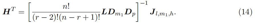
Note that empirically the above matrix is testable since the joint probability matrix can be estimated directly from the data. This full rank condition can be guaranteed that the type-specific bid distributions are linearly independent. The full rank assumption leads to the following main equation for identification:

where Dm1/m2 is a diagonal matrix
with the kth diagonal element as the ratio of the probability that type k occurs in two middle intervals m1 and m2, i.e.,
Equation (9) indicates that the observed matrix on the left-hand side and the unknown matrices on the right-hand side are similar. Specifically, the probability matrix involved the “low” support L and the probability ratio matrix involved the “‘middle” support Dm1/m2 can be identified as the eigenvector and eigenvalue matrices of the observed joint probability matrix. Unique decomposition requires a condition that the diagonal elements differ from each other, as in the following assumption.
Assumption 2. (Distinctive Eigenvalues)
There exist a mapping from xr−1 to two intervals of the “middle” support m so that the ratio of the probability that the type- specific underlying random variable falls into the two intervals differ for any two types.That is,
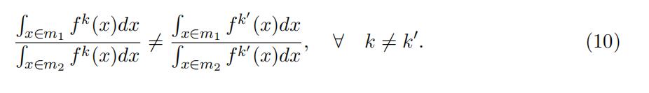
This assumption is empirically testable
since we can estimate the eigenvalues directly from the decomposition and can be achieved by choosing the cutoff point of the sup- port. With the assumptions of full rank and distinctive eigenvalues, we can identify the probability matrix involved the “low” support L, whose kth column is the probabilitythat the order statistics Xkr−2:r−2 falling in the K intervals {l1, …., lK} up to relabeling and scales. Note that the probability matrix involved the “low” support (L) is identified as the eigenvector matrix through an eigenvalue and eigenvector decomposition. As a result, L is identified up to scales and relabeling.
Identification up to scale
is a prevalent feature of identification using the mixture feature. Pinning down the scale requires a normalization condition. In the existing liter- ature of independent measurements, a normalization condition could be that the column sum equals 1 because it represents a total probability. This normalization condition is not applicable here because the column sum is not a total probability anymore after we divide the whole support into three portions. We will keep this identification up to scale for now and provide restrictions to pin down the scales later.
With this identified probability matrix involved the “low” support,
we can furtheridentify the density for the order statistics Xkr−2:r−2 for any value in this interval. Then we can use the connection between the density of an order statistics and the density of the original distribution to recover the type-specific density distribution for the “low support. In particular, to identify the density for the order statistics Xkr−2:r−2, we again use the joint distribution. Note that, the matrix representation in equation (8) also holds for a particular value of xr−2 = x ∈ l. Thus, we have
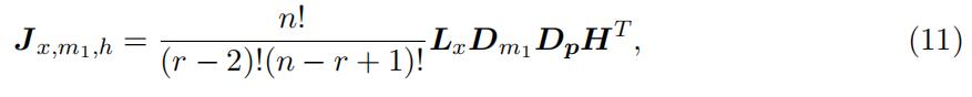
where Jx,m1,h and Lx are the counterparts of matrix Jl,m1,h and L with replacing the interval to a particular value of xr−2 = x ∈ l, respectively, so that Lx represents density. Note that both equation (8) and the above equation have common components Dm DpHT , which is invertible. Consequently, we can identify the type-specific density for order statistics Xkr−2:r−2 in the “low” support, i.e., f kr−2:r−2(x), ∀x ∈ l,
as in the following closed-form expression:

Note that the density vector Lx is identified up to the same scales and ordering of the probability matrix L.
Now we proceed to identify the type-specific density using the identified type-specific distribution of the order statistics f kr−2:r−2(x) in the “low” support through the following closed-form expression.
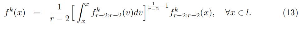
Again the type-specific density is identified up to scales since the type-specific density of order statistics Xkr−2:r−2is identified up to scale. Note that the two scales might differ.
We summarize the above results in the following Lemma and leave the proof details in the Appendix.Order Statistics代写
Lemma 1 Order Statistics代写
(low support). If Assumptions (1) and (2) are satisfied, the type-specific density in the “low” support, i.e., f k(x), ∀x ∈ l, is identified up to scales.
In what follows, we identify the type-specific density function f k(x) in the “high” support. Specifically, we first identify the probability matrix H involved the “high” support up to scales using the joint distribution in equation (8):
Since L is identified up to scales due to the decomposition, and both Dm1 and Dp are diagonal matrices, H can be identified up to scales, but the scales are different from the scales in L.
We then can follow
the same identification argument in lemma 1 to identify the type-specific probability density for order statistics f k1:n−r+1(x) by replacing the bins in h by a particular value x ∈ h and use invertibility of the matrices to cancel out common components. We then use the connection of the type-specific density for order statistics and the type-specific density function to recover the type-specific density. In particular,

Note that f k1:n−r+1(x) is identified up to scales, so the type-specific density f k(x)∀x ∈ h is also identified up to scales. We summarize this identification result in the following Lemma.Order Statistics代写
Lemma 2
(high support). If Assumptions (1) and (2) are satisfied, the type-specificdensity in the “high” support, i.e., f k(x), ∀x ∈ h, is identified up to scales.
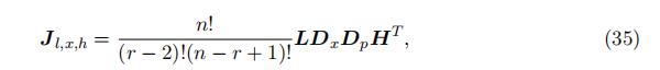
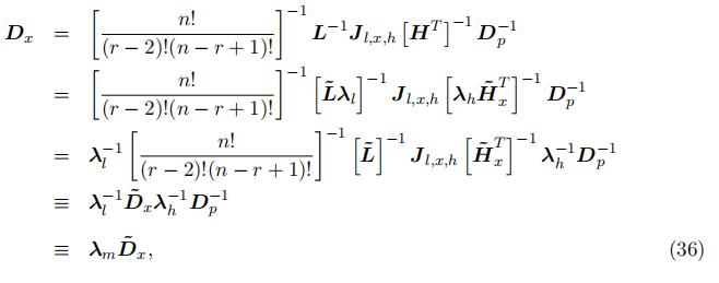
With the type-specific density function being identified for the “low” and “high” support, we now move to identify the density in the “middle” suport. The identification again is similar as in lemma 2. We again rely on the joint distribution relation similar in in equation (8), leading to the following matrix representation:

where Jl,x,h and Dx are the counterparts of matrix Jl,m1,h and D with replacing the interval to a particular value of xr−1 = x ∈ m, respectively. Note that L and H are both identified up to scales and Dp is a diagonal matrix. As a result, Dx can be identifiedup to scales, with the kth diagonal element being the type-specific density f k(x) where x ∈ m.
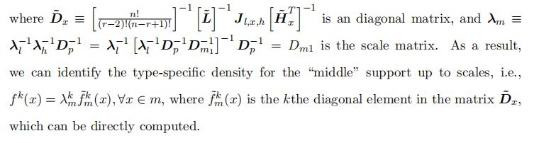
Lemma 3 Order Statistics代写
(middle support). If Assumptions (1) and (2) are satisfied, the type-specific density in the “middle” support, i.e., f k(x), ∀x ∈ m, is identified up to scale.
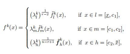
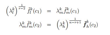
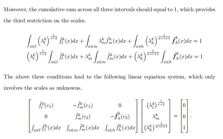
Note that we identify the type-specific density f k(x) for the “lower”, “middle”, and “high” portion up to different scales, which requires three conditions to pin down the scales exactly. First, the three density functions identified separately should be the same at the cutoff points c1 and c2 for the two densities overlapping in the cutoff points.Order Statistics代写
Moreover, the fact that the cumulative sum across all three intervals should equal to 1, which provides the third restrictions on the scales. Once the scales being pinned down, we can identify the type-specific weight pk.Order Statistics代写
To sum up, we can identify the type-specific bid distribution using only three consecutive order statistics of the bids. With the type- specific bid distribution being identified, we then can identify the type-specific value function in both first price or second price IPV auctions when the number of potential bidders is known. We summarize all results in the following theorem.
Theorem 1.
If the competition n is known and Assumptions (1) and (2) are satisfied in IPV auctions, the type weight pk, the type-specific bid distribution f k(x) for x ∈ [x, x¯k], and the type-specific value distribution Φk(v) for v ∈ [v, v¯k] are identified for all k using three consecutive order statistics.
This result relies on the consecutiveness
of the three order statistics and the above eigendecomposition strategy. Although we believe observing consecutive order statistics is common, our identification strategy applies to arbitrary order statistics if there are four. First, the joint density is separable by conditioning on the second and the third order statistic.
This step uses the Markov property of order statistics. See also Mbakop (2017). Second, we can construct an eigendecomposition structure using this joint den- sity at four pairs of the two middle order statistics. This strategy is similar to some recent results on identification of dynamic models with unobserved state variables (Hu and Shum (2012) and Luo, Xiao, and Xiao (2018)). Third, we follow a similar strategy as above to identify the component distributions in a lower portion of the support and then in an upper portion.
Identification using two consecutive order statistics with an instrument Order Statistics代写
In some scenarios, we might only observe only two consecutive order statistics, such as the top 2 bids, in which case the above identification results cannot be applied. In this scenario, an extra instrument for the UH would work as well as the third order statistics and enables identification of the type-specific bid distributions in a similar manner using the joint distribution of the two consecutive order statistics and the instrument.
An instrument is a variable that is independent with the order statistics conditional on the type. Furthermore, the requirement for the instrument is mild, in the sense that as long as there is variation in the instrument, such as binary, the identification argument below can go through.3
3This is similar to the Hu (2017) 2.1 measurement model.
Suppose we observe two consecutive order statistics of the n ordered sample Xr−1:n, Xr:n and an instrument Z, where Z ∈ {0, 1}. The joint distribution of these three variables are
Similarly, we divide the space into two exclusive intervals and further discretize both intervals into K exclusive intervals. Fix z = 0, we can rewrite the above equations con- necting the unknown type distribution with the observed joint probability into a matrix representation. We also can rewrite the joint distribution of the two order statistics in a similar matrix manner. We thus can follow the previous identification argument to identify the type-specific distributions.
3.3 Identification using two order statistics with support variations Order Statistics代写
In auctions with UH, sometime the UH not only are drawn from different distributions, but also shifts the support of bids, which provides useful variations for identification. The variation in supports essentially reduce the mixture components in some regions of their supports. This subsection shows that with support variations, two arbitrary order statistics, instead of three consecutive ones, are sufficient to identify the unobserved distribution. Specifically, suppose we observe two order statistics Xr:n and Xs:n of bids,where r < s, for a n ordered sample. Note that fr,s:n(xr, xs) = Σkk r,s:n (xr, xs) andfs:n(xs) = Σkk s:n(xs).
We first formally introduce the support variations in the following assumption.
Assumption 3.
(Support variations) x1 < x2 <, . . . , < xK.
To illustrate the role of the support variations play in the identification, we display the support of the joint PDF for the order statistics {Xs:n, Xr:n} in Figure 4. We assume that K = 3 for illustration purpose. First, the support is below the 45 degree line because Xs:n ≥ Xr:n by definition.
Second, there is a jump in density at every upper bound of type xk because the density for lower types vanishes. Specifically, the light red areas between x2 and x3 involves only the highest type k = 3, i.e., the mixture feature degenerates; the middle area involves only the top two types, k = 2, 3, i.e., the mixture only have two components instead of three; only the dark red area between x and x1 involves all three types.
Figure 4: Support of the Joint PDF for (Xs:n, Xr:n)
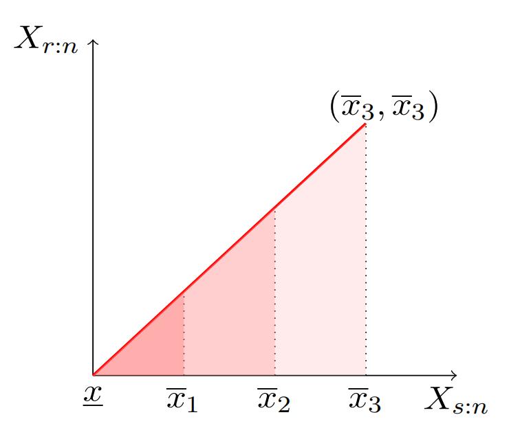
We show the identification of type-specific distribution using this support variation sequentially. First, we identify the distribution of the highest type using the fact that the observed distribution in the area of xK−1 and xK provides information only about type K.
Then we recover type k’s distribution by excluding the identified higher type k + 1, …K from the observed distribution in the area of [xk−1, xk], which only involves distributions of type k = 1, …, K. We summarize the whole identification in the following two Lemmas.
Lemma 4.
If Assumption 3 is satisfied, the bid distribution of the highest type F K(·)and weight pK are identified.
Consider xs:n = xs ∈ (xK−1, xK], the conditional density function of xr given xs is
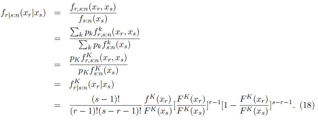
The third equality holds because the area of (xK−1, xK] only concerns type K. This conditional density is the density function of rth order statistics from a sample of size s−1 from a distribution F K(·) truncated on the right at xs.4 Let xs = xK.
The truncation
is no longer effective. We then further simplify the conditional density function as

where fKr:s 1(·) is the density function for rth order statistics from a sample of size s 1(·) is the density function for rth order statistics from a sample of size s − 1with a distribution F K(·). This implies that F K (·) is identified. Thus, F K(·) isidentified following footnote 1.
Moreover, the weight for type K can be identified through a marginal distribution in the area of any xs ∈ (xK−1, xK]. That is,

4Song (2004) identifies a model for eBay auctions using a different property that fs|r:n(·) is the sameas the density of (s − r)th order statistics from a sample of size (n − r) from F (x) truncated on the left at xr . However, his considers homogeneous auctions where only the number of bidders varies. Moreover,his focus was the identification of the value distribution.
With the distribution of the highest type being identified, we next identify the distribu- tion of the remainning types using iteration induction, stated in the following Lemma.Order Statistics代写
Lemma 5.
If F k(·) and pk are identified for all k = kˇ + 1, . . . , K, F kˇ(·) and pˇare identified.
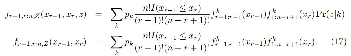
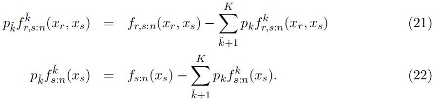
We again use the joint distribution and consider xs:n = xs ∈ (xkˇ−1, xkˇ]. Note that this areas only involves higher types k = kˇ, . . . , K. In this specific area, we can represent the joint distribution of the two order statistics and the marginal distribution as
Since the distribution and weight of the higher types are identified, we can identify the distribution of type kˇ through excluding the identified components from the observed counterparts.
Consequently, following the identification argument in Lemma 4, we can identify the conditional density function of xr given xs of type kˇ through the following equatios

Similar to above, we obtain
which identifies F kˇ(·) and thus F kˇ(·). Moreover, pˇ = pˇf kˇ(xs)/f kˇ(xs). In sum-r:s−1k k s:n s:n mary, the distribution function and weight for type kˇ can be identified.
Lemmas 4 and 5 imply that the distributions F k(·) and weight pk are nonparamet- rically identified. In auction models, we can identify the type-specific bid distributions using the support variation. Consequently, we can identify the type-specific value dis- tributions in IPV auctions.
Theorem 2. If the competition n is known and Assumptions 3 is satisfied, the weight of type pk, the type-specific bid distribution F k(x), and the type-specific value distribution Φk(v) in IPV auctions are identified for all k using any two order statistics.
Identification with multidimensional UH in first price auction Order Statistics代写
We extended the above identification argument to first price auctions with two sources of UH: unobserved auction type k and unobserved competition n. We assume that the number of bidders n is exogenous and the maximal number of potential bidders N is known. We first relabel the type as ω = (k, n). In a first-price auction, each type (k, n) maps with a type-specific value distribution Φk(v) and corresponds to a bid distribution F k,n(x)that has support [x, x(k,n)]. We now study how to identify the value distributions Φk(·) and the distribution of each type p(k,n).
Similar to the previous section, in first price auctions,
a sufficient condition for the support variation (Assumption 3) is that the type-specific value distribution has a first- order stochastic dominance relation (FOSD).
Assumption 4. (FOSD) Φ1(v) ≤ Φ2(v) ≤ . . . ≤ ΦK(v) for all v, with strict inequality at some v for each pair of the value distributions.The FOSD condition not only generate support variation for the unobserved type k with a given n, it also provides support variation for the competition n with a given k.Giventhat Assumption 4 is satisfied, Guerre, Perrigne, and Vuong (2009) and Hu,McAdams, and Shum (2013) discuss how the upper boundary varies with respect to n and k, respectively.
Lemma 6. Order Statistics代写
For a given k (n), the upper boundary x(k,n) is strictly increasing with respect to n (k) if Assumption 4 is satisfied.
Lemma 6 shows that there is a jump at each upper boundary xω. Without loss of generality, let 0 < ω1 < ω2 < . . . < ω2K. These points divide the support of x(w) into K × (N − 2) intervals. The top portion (xω2K−1 , xω2K ] corresponds to highest UH and the biggest number of bidders ω = (K, N ).
Following the same lines in Section 3.3, we can identify the weight and bid distribution associated with the highest types, i.e., p(K,N ) and F K,N (·), respectively. Consequently, we can identify the value distribution associated with the highest type, ΦK(·).Moreover, we can use ΦK(·) to identify the upper boundary x(K,n) and the corresponding bid distribution function F(K,n)(·) for all n < N .
We then proceed to identify the type-specific bid distribution F k,n(·),
weight p(k,n), and type-specific value distribution Φk(·), for all k < K and all n, using iteration induc-tion. Specifically, we show that p(kˇ,n), F kˇ,n(·), and Φkˇ(·) are identified if p(k,n), F k,n(·),and Φk(·) are identified for all k = kˇ + 1, . . . , K. Excluding x(k,n) for all k > kˇ and all n,
we find the maximum of the other jump points. Lemma 6 implies that this point corresponds to (k, n) = (kˇ, N ). Again, we follow Guerre, Perrigne, and Vuong (2000) to identify the associated type-specific value distribution Φkˇ(·). We then use the identi-fied type value distribution Φkˇ(·) to identify the related bid distribution function with different competition levels F kˇ,n(·), for all competition n.
Theorem 3. If Assumption 4 is satisfied, the weight pk,n, the bid distribution F k,n(·), and the value distribution Φk(·) are identified for first price IPV auctions with unobserved type k and unknown competition n using any two order statistics.
4 Identification with Separable UH Order Statistics代写
This section considers the generic identification of separable UH in auction models. Fol- lowing the existing literature, we assume that the auction-level UH enters in individual bidders’ value in an additively separable fashion. Specifically, we consider auctions where individual bidder’s value comes from two parts:
Vi = V ∗ + ui, (24)
where V ∗ is the auction-level UH and ui are the idiosyncratic part. See, e.g., Li, Perrigne, and Vuong (2000). The distribution of UH and the private part are denoted as ΦV ∗ (·)
with support [v, v¯] and Φu(·) with support [u, u¯], respectively. We first impose the mutually independent assumption as in the existing literature.
Assumption 5.
(Independence) The common value V ∗ and the idiosyncratic value shocks ui are mutually independent. Moreover, ui are i.i.d. conditional on the auc- tion heterogeneity V ∗.
With the independence condition, we can further represent the observed bid Xi in the same additively structure in the following, as shown in Haile, Hong, and Shum (2003).Xi = X∗ + si, (25)where X∗ and si map to the value V ∗ and ui, and their distributions denoted as FX∗ (·) with support [x, x¯] and Fs(·) with support [s, s¯], respectively. Moreover X∗ = V ∗.We now provide sufficient conditions to identify both distribution functions FX∗ (·) and Fs(·) using the joint distribution of the top two order statistics of the bids when the competition n is known, i.e., Xn:n and Xn−1:n.
We then extend the identificationOrder Statistics代写
5In the case of multiplicative separability, Vi = V ∗ui, where V ∗, ui > 0. We can apply logarithm on both side to obtain an additive separable form log Vi = log V ∗ + log ui.argument to the scenario of any two consecutive order statistics. Note that the usual approach that exploits the joint characteristic function (Li, Perrigne, and Vuong (2000)), no longer applies because order statistics are dependent by definition and thus the joint characteristic function is no longer multiplicatively separable in individual ones. Despite this, Athey and Haile (2002) conjecture that there is enough structure to identify the model from two order statistics.
However, there has been no such result in the literature.6
One natural approach is to take the difference between two order statistics and study identification of the parent distribution from the distribution of this spacing. However, this approach does not necessarily work. For instance, Athey and Haile (2002) point out a counterexample in Rossberg (1972): if X1, X2 are i.i.d. random variables with F (x) = 1 − e−x[1 + π−2(1 − cos 2πx)] on support R+, the spacing X2:2 − X1:2 has astandard exponential distribution.
Our identification procedure
also relies on characteristics function of the order statis- tics but exploit the “within” instead of the “between” independence. In particular, al- though sn−1:n and sn:n are dependent, we can exploit the fact that X∗ ⊥ sn−1:n and X∗ ⊥ sn:n. We now introduce some notation. We use ψX (t) to denote characteristic function for a random variable X. Order Statistics代写
For ease of notation, let snˇ:nˇ≡ max{s1, . . . , snˇ},where nˇ= n, n − 1, . . . , 1, which is the top order statistics of i.i.d. random draws from a parental distribution Fs(·); Let ψnˇ(t) denote snˇ:nˇ’s characteristics function, so ψnˇ(t) = ∫ +∞ exp[i(ty)] · [nˇF nˇ−1(y)fs(y)]dy.7
We first identify the ratio of the characteristics function of the top order statistics from a n − 1 and n ordered sample using the characteristics function of the observed order statistics, i.e., ψn−1(·)/ψn(·).
Lemma 7.
If Assumption 5 is satisfied, the ratio of the characteristics function of the 6Freyberger and Larsen (2017) have a similar problem with eBay auctions but they circumvent the issue of correlated order statistics using observed reserve prices, rendering the identification problem classical.
7Note that ψ1(t) = ψs(t).top order statistics from a n and n − 1 ordered sample, i.e., ψn−1(t)/ψn(t), is identified. Proof. Under Assumption 5, UH and the order statistics of the idiosyncratic parts are also mutually independent.
That is,
ψXn:n (t) = ψX∗ (t) · ψsn:n (t) = ψX∗ (t) · ψn(t), (26)
ψXn−1:n (t) = ψX∗ (t) · ψsn−1:n (t) = ψX∗ (t) · .nψn−1(t) − (n − 1)ψn(t)Σ. (27)
Cancelling out the characteristics function of the common UH leads to the following equation
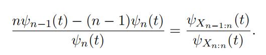
Consequently, we can identify the ratio of the characteristics function of the two top order statistics as

Now we proceed to identify the distribution Fs(·) using the identified ratio of the characteristics functions of the two top order statistics ψn−1(t)/ψn(t). Note that both support for X∗ and s is unknown, i.e., [x, x¯] and [s, s¯] are yet to identify together with their corresponding distributions. Consequently, it is observational equivalent if we adda constant to X∗ and subtract the same amount from si. We make the following location normalization for ease of exposition.8Order Statistics代写
Assumption 6. (Normalization) s = 0.
8The existing literature with independent measurements assumes that it is mean zero. See, e.g., Li, Perrigne, and Vuong (2000). Our normalization is without loss of generality.
We first define identification formally in this context.
Deftnition 1.
(Identification) The distribution of the idiosyncratic part Fs(·) is identi- fied if any two distribution functions F (·) and tt(·) are the same once they satisfy the following two conditions:
1.their supports are of the form [0,s]9;
2.theyhave the same ratio of the characteristic functions of the two top order statis-
tics, i.e., ψn−1(t) = ψnj −1(t) , where ψn−1(t)and ψnj −1(t)are associated with F (·) and ψn(t)tt(·), respectively.ψnj (t)ψn(t)ψnj (t)
Note that ψn−1(t)/ψn(t) = ψnj −1(t)/ψnj (t) is equivalent to ψn(t)ψnj −1(t) = ψn−1(t)ψnj (t).
Consequently, the identification problem is equivalent to the following problem.
Problem 1. Xi’s and Yi’s are i.i.d. random variables with distribution function F (·) on support [0, s¯F ] and tt(·) on support [0, s¯tt], respectively. Let Z1 = Xn:n + Yn−1:n−1 and Z2 = Xn−1:n−1 + Yn:n.10 Identification in our context is equivalent to the situation that Z1 and Z2 have the same distribution implies that F (·) = tt(·) and s¯tt = s¯F .
We now proceed to prove that Z1 and Z2 have the same distribution implies that s¯tt = s¯F and F (·) = tt(·), so that our original auction structure is identified. Specifically, by the convolutions of probability,
Z1 has a density function
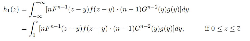
where s¯ = min{s¯F , s¯tt}, and nF n−1(·)f (·) and (n − 1)ttn−2(·)g(·) represent the density functions of Xn:n and Yn−1:n−1, respectively.
9Their supports are unknown to the analyst and might be different.
10Note that Z1 and Z2’s have support [0, g¯F +g¯G] and their characteristics functions can be represented as ψn(t)ψnj −1(t) and ψn−1(t)ψnj (t), respectively, because X’s and Y ’s are independen.
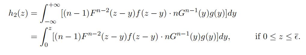
Similarly, Z2 has a density function
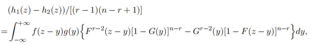
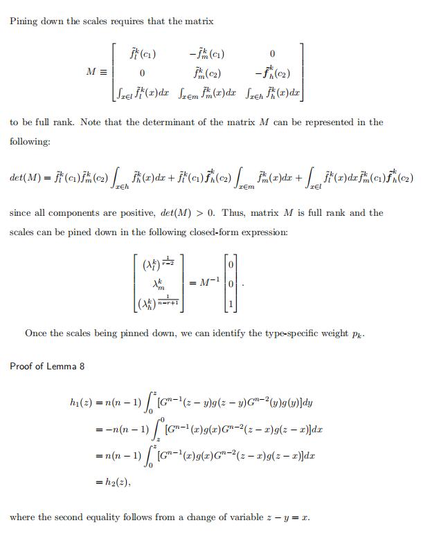
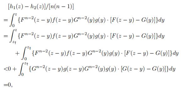
Lemma 8.
For any z ∈ [0, s], if F (t) = tt(t) for all t ≤ z, h1(z) = h2(z).
To show that the distribution Fs(·) is identified, we rely on an Restricted Stochastic Dominance ordering (RSD) assumption introduced in Luo (2018). That is, fs(·) belongs to the set of density functions in which any two functions can be ranked using RSD ordering (Assumption 7).11
Assumption 7. (RSD) g(·) dominates f (·) in the restricted sense if there exists an
y > 0 such that: (a) f (s) ≥ g(s) for all s ≤ y, and (b) ∃y∗ ≤ y, f (y∗) > g(y∗).
Lemma 9. Under Assumption 7, h1(·) = h2(·) implies that F (·) = tt(·) and s¯tt = s¯F .
Lemma 9 implies that Fs(·) is identified once the ratio ψn−1(·)/ψn(·) is identified. Consequently, the distribution of X∗, FX∗ (·) is identified. With the identified distribu- tion FX∗ (·) and Fs(·), following the arguments in Section 2, we can identify the distri- butions of UH and private value.12
Identification with any two consecutive order statistics
We further extend the above argument to the scenario of any two consecutive order statistics, Xr−1:n and Xr:n. Denote the distribution of X as F (·).
11It is worthnoting that the counterexample of Rossberg (1972) satisfies this condition and thus our characteristic function approach identifies the parent distribution. In fact, f (x) − e−x = e−xπ−2[1 − cos 2πx − 2π sin 2πx], which approaches 0 when x ↓ 0. Moreover, the slope of the difference is negative at x = 0. Therefore, there exists an x† such that f (x) < e−x, x (0, x†).
12Lemma 8 and Lemma 9 extend to the case with a maximum order statistic Xm:m and any other order statistic Xr:n, where m > r or m = r < n.
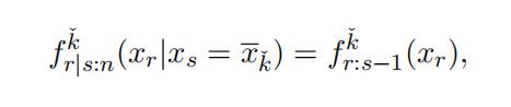
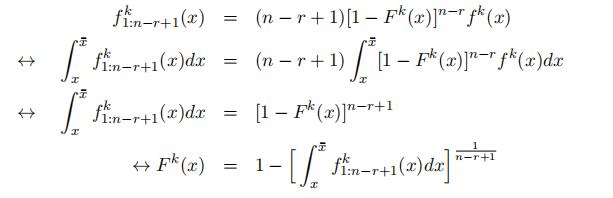
First, note that for any (n, r), we can observe the conditional density functions of one order statistic given a consecutive one and they satisfy the following conditions:
f˜−1|r:n(xr−1|xr = x) = f˜r−1:r−1(xr−1),
f˜|r−1:n(xr|xr−1 = x) = f˜1:n−r+1(xr),
which identify fr−1:r−1(·) and f1:n−r+1(·), respectively.Order Statistics代写
Second, following Lemma 7, the corresponding characteristic function are ψr−1:r−1(t) = ψX∗ (t)ψr−1:r−1(t) and ψ1:n−r+1(t) = ψX∗ (t)ψ1:n−r+1(t), respectively. ψr−1:r−1(·) and ψ1:n−r+1(·) represent the characteristic functions of two order statistics sr−1:r−1 and s1:n−r+1, respectively. Therefore, we can identify the ratio
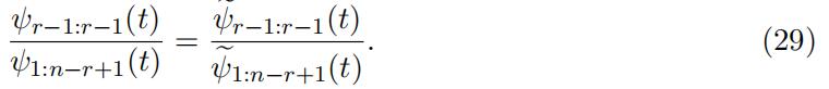
Similar to above, the identification problem can be restated as
Problem 2. Xi’s and Yi’s are i.i.d. random variables with distribution function F (·) on support [0, s¯F ] and tt(·) on support [0, s¯tt], respectively. Let Z1 = Xr−1:r−1 + Y1:n−r+1 and Z2 = X1:n−r+1 + Yr−1:r−1. Identification in our context is equivalent to the situation that Z1 and Z2 have the same distribution implies that F (·) = tt(·) and s¯tt = s¯F .
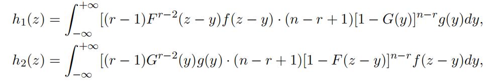
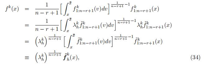
The density functions of the minimum X1:n−r+1 and the maximum Xr−1:r−1 are
f1:n−r+1(x) = (n − r + 1)[1 − F (x)]n−rf (x),
fr−1:r−1(x) = (r − 1)F r−2(x)f (x),
respectively. Therefore, the density functions of Z1 and Z2 are
respectively. This implies that
which is increasing with respect to f and F when the quantity in the curly brackets is positive. The rest follows similar arguments as Lemma 8 and Lemma 9.
Theorem 4. If Assumptions 5 – 7 are satisfied and the competition is known, the dis- tribution of the auction-level UH and the idiosyncratic part ΦV ∗ (·) and Φu(·) in IPV auctions are identified using two consecutive order statistics of the bids.
5 Empirical Application: USFS timber second-price auctionsOrder Statistics代写
In this section, we apply our identification results to an empirical analysis of the United States Forest Service (USFS) timber auctions. Other studies of these auctions include Baldwin, Marshall, and Richard (1997), Haile (2001), and Haile and Tamer (2003). Related to our setting, Aradillas-L´opez, Gandhi, and Quint (2013) consider a more general model and apply a bound approach to the English auctions, which is the first to study these auctions allowing for correlated values. This paper focuses on independent private values with UH and achieves point identification and estimation.
5.1 Institution Background and Data
Timber is one of the most important outputs from National Forests managed by USFS. Auctions are used to allocate the right to harvest from tracts. These tracts are highly heterogeneous. USFS publishes a cruise report that provides information about the tract being auctioned in narrative form. It includes one or more maps showing features of the tract, a discussion of all harvesting cost expected (such as transportation), and conditions of sales (such as planned cutting methods, protective measures for controlling erosion, and contract provisions) et al.
The government uses three methods of sale: English auction, sealed-bid first price auction, and noncompetitive method. We will focus on Enligh auctions, which are conducted in two rounds: a sealed bid auction is followed by oral bidding unless only one sealed bid was received.
Data Sample Order Statistics代写
In particular, we analyze the ascending English auction data from 1982 to 1990, which are constructed from the data available on Professor Philip A. Haile’s website.13 Fol- lowing the seminal paper Haile, Hong, and Shum (2003), we consider only scaled sales in Forest Service Regions 1 and 5 to minimize the significance of subcontracting/resale and thus common value. Moreover, we drop salvage sales and sales that are set aside for small businesses. In summary, we focus on auctions that are most likely to satisfy the independent private value assumption. In total, we have 1207 ascending English auctions.
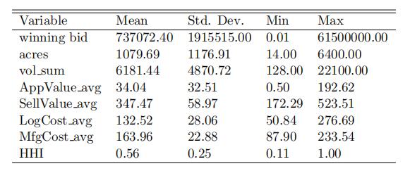
Table 1 provides some summary statistics on auction-specific covariates:
winning bid, size of tract (in acres), estimated volume of timber (in MBF), appraisal value (per MBF), estimated selling value (per MBF), estimated harvesting cost (per MBF),estimated manufacturing cost (per MBF), and species concentration index (HHI). We construct these covariates following Liu and Luo (2017). All dollar values are nominal and all volume values are in thousand board feet (MBF) of timber.
13http://www.econ.yale.edu/ pah29/timber/timber.htm
Table 1: Summary Statistics
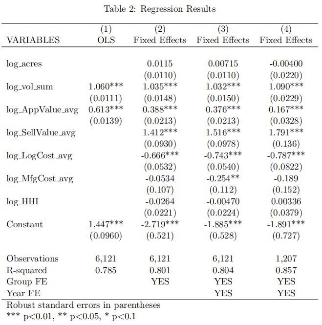
Before applying our methodology, we implement the Haile, Hong, and Shum (2003) method to homogenize the bids. Table 2 displays the regression results. Regressions (1)-(3) use all bids but different control variables. All estimated coefficients have the expected signs. Regression (3) includes all control variables as well as year dummies. As argued above, it is more suitable to model top bids as order statistics. See also Aradillas-L´opez, Gandhi, and Quint (2013).
Moreover, multiple top bids (and their “homogenized” counterparts) Order Statistics代写
from the same auction are correlated by definition, leading to biases in the estimated coefficients. Therefore, we use only the winning bid to control for auction-specific covariates. Regression (4) is the same as (3) but using only winning bids. All estimated coefficients have the expected signs. Moreover, the regression with only winning bids shows a much better fit than the other ones. Lastly, we calculate homogenized bids as the exponential of the differences between the logarithm of the original total bids and the demeaned fitted values of Regression (4).
In the following analysis, we only use the top three “homogenized” bids.
5.2 Empirical Results Order Statistics代写
To make sure the bids are informative for the value, we exclude the bids that are very closed to the estimated prices by USFS. Furthermore, the highest bid and the second highest bids are quite close to each other, both revealing information on the second highest value among all the bidders.
Thus, we use the transaction price as the 2nd highest value among all the bidders and exclude the 2nd highest bid from the data to avoid redundant information for the 2nd highest values. We then use the 3rd and 4rd bids as the proxies to the 3rd and 4th highest values among all the bidders. Note that from the identification, we need to have at least three informative bids, which means at least four bids from the data. We have 496 auctions.
We use beta distributions
to approximate the underlying type-specific component distributions and estimate the type-specific beta coefficients and the corresponding type probability using a maximum likelihood estimator.14We estimate the underlying com- ponent distribution and the type probability for the number of types being three, i.e., ‘low’, ‘middle’, and ‘high’.
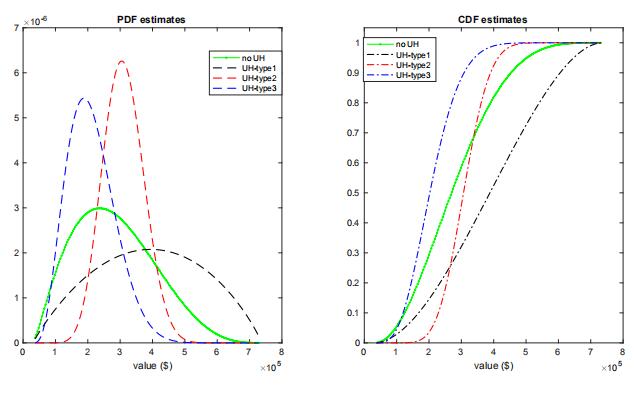
The probability for the three types is 0.24, 0.37, and 0.39, respectively. Each type accounts for a nontrivial portion of the sample, confirming the importance of allowing for UH in our analysis. We present the estimated type-specific pdf and cdf for values in figure 5 for the case allowing for UH and the case without UH. As noted in Krasnokutskaya (2011), ignoring UH leads to a biased estimate of the value distribution with an overestimated dispersion.
Figure 5: Estimation of PDF and CDF: no UH vs UH
14We have also conducted Monte Carlo experiment with a semi-parametric estimator using sieve approximation. The estimator performs quite well with a moderate number of sample size. The results are available upon request.
Bidder Surplus and Expected Revenue
With the estimates of value distributions, we compute the bidder ex ante expected surplus and auctioneer’s expected revenue to provide a comparison between the cases of no UH and UH and present the results in figure 6. The solid (dashed) lines represent the results with (without) UH. Black (purple) lines represent the results without (with) the reserve price. The black lines in the left-hand figure suggests that we overestimate bidder expected surplus if UH is ignored.
Note that in auctions with less disperse values, a likely winner who has a high value expects the other bidders to have similar high values with a higher probability. Therefore, bidders tend to be more aggressive. When attributing wrongly the variation in UH to bidders’ values, we overestimate bidder heterogeneity and underestimate bidders’ aggressiveness.
As a result, we overestimate bidder expected surplus.
The black lines in the right-hand figure suggests that ignoring UH leads to underestimation of expected revenue when the number of bidders is small and overestimation otherwise. Consider the number of bidders n = 2. The bidder’s surplus is around $ 70,708 and $ 50,957 for model estimates without and with UH, respectively; the seller’s revenue is around $ 211,717 and $ 238,590 for model estimates without and with UH, respectively.
Next, we examine the effects of an optimal reserve price on bidder surplus and sellerrevenue. Reserve price is the minimum amount that the seller will accept as the winning bid. In a second-price auction, a reserve price does not change bidders’ optimal bidding behaviors. Note that the black line and the purple line converge when the number of bidders increase.
In other words, an optimal reserve price makes less difference in larger auctions.
Nevertheless, most auctions have very few bidders and thus the choice of a reserve price is empirically relevant.Consider again the number of bidders n =2.Using the estimated model with UH, the optimal reserve prices are $ 321,100, $ 239,400, and $ 155,100, respectively, which corresponds to a probability of no biddin of0.36,0.13, and 0.24, respectively. The mode of the type-specific value distribution is
Figure 6: Bidder surplus and expected revenue
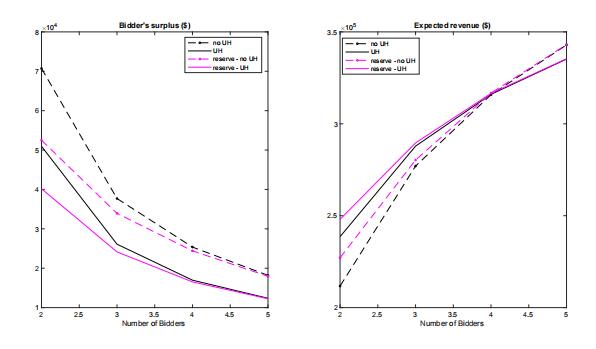
$ 394,396, $ 304,871, and $ 187,971, respectively. The optimal reserve prices lead to an ex-ante expected bidder surplus of $ 40,187 and seller revenue of $ 248,025. Using the estimated model without UH, the optimal reserve price is $ 219,800, which corresponds to a probability of no bidding of 0.35. The mode of the value distribution is $ 236,786. This optimal price leads to an ex-ante expected bidder surplus of $ 52,498 and seller revenue of $ 227,113. Therefore, ignoring UH leads to substantial bias in the optimal reserve price policy and welfare estimates.
6 Conclusion Order Statistics代写
Auction data often fail to record all bids or all relevant auction-specific characteristics that shift bidder values. Instead, they contain only order statistics of bids and suffer from unobserved heterogeneity. In this paper, we present a set of new identification results for auction models with UH using order statistics. In particular, we show that, despite being dependent, the same number of order statistics as that of the independent measurements are sufficient to achieve similar identification results for both discrete and continuous UH. Our results rely on consecutive order statistics or support variations.
7 Appendix Order Statistics代写
7.1 Proof of Theorem 1
This subsection provides derivation of all the necessary conditions for Theorem 1.
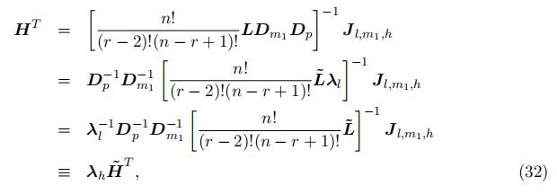
Proof of Lemma 1: identification in the “low” support The full rank assumption leads to the following main equation for identification:
![]() where Dm1/m2 is a diagonal matrix with the kth diagonal element as the ratio of the probability that type k occurs in two middle intervals m1 and m2, i.e., ,x∈m1f k(x)dxk. With the assumption of distinctive eigenvalues, we can identify the probability matrix involved the “low” support L as the eigenvector matrix through an eigenvalue and eigenvector decomposition.Order Statistics代写
where Dm1/m2 is a diagonal matrix with the kth diagonal element as the ratio of the probability that type k occurs in two middle intervals m1 and m2, i.e., ,x∈m1f k(x)dxk. With the assumption of distinctive eigenvalues, we can identify the probability matrix involved the “low” support L as the eigenvector matrix through an eigenvalue and eigenvector decomposition.Order Statistics代写
Note that the components identified from the eigenvalue-eigenvector decomposition are not the probability matrix L itself, but the matrix L with each column multiplied by an unknown constant. That is, denote the eigenvector matrix obtained from the
decomposition L˜, we have L = L˜λl, where λl ≡ diag[λ1, …, λK] is the scale matrix.
Basing on the matrix L˜from the decomposition, we can compute the corresponding density matrix through equation (12)
As a result, the type-specific density for order statistics Xkr−2:r−2 in the “low” sup-port is identified up to the same scale as the probability matrix L, i.e., f k
r−2:r−2(x) =λkf˜k(x), where f˜k(x) is the kthe element in vector L˜x.
We then move forward to show that the type-specific density f k(x) is also identified up to scales in the follows.
Thus, we can derive the type-specific density for x ∈ l as in the follows.
where ![]() represents the type-specifific density computed using the eigenvector matrix directly from the decomposition, which is known. The type-specifific density in the “low” support is identifified up to scale of
represents the type-specifific density computed using the eigenvector matrix directly from the decomposition, which is known. The type-specifific density in the “low” support is identifified up to scale of ![]()
Proof of Lemma 2: (identification in the “high” support) In what follows, we identify the type-specific density function f k(x) in the “high” support.
First of all, we can identify the probability matrix H up to scale from the joint distribution equation (8) as the following closed-form expression:
where λh ≡ λ−1D−p 1D−1 ≡ diag{λ1 , …, λK} is a diagonal matrix captures the unknown scales, and H˜ T represent the component that can be computed using result from the decomposition. Since L is identified up to scales due to the decomposition, and both Dm1 and Dp are diagonal matrices, H can be identified up to scales, but the scales are different from the scales in L.
We then can follow the same logic to identify the type-specific density for the “high”support.
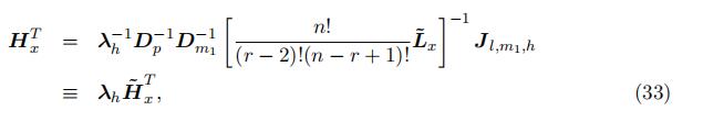
where HTand H˜ T are defined similar to HTand H˜ T, respectively. This indicates
that the type-specific density in the “high” support can be identified up to scale, i.e.,
f k (x) = λkf˜k(x), where f˜k ˜ T1:n−r+1 h 1:n−r+11:n−r+1(x) is the kth component in the vector Hx ,which can be computed using results from the decomposition.
We then use the connection of the type-specific density for order statistics and the type-specific density function to recover the type-specific density. In particular, for any value in the “high” support, i.e., x ∈ h,
by definition of the order statistics, we have
Thus, we can link the type-specific density to the type-specific density of the order statistics in the follows, ∀x ∈ h:
The type-specific density in the “high” support is identified up to scale of .λkΣ 1 .
Proof of Lemma 3: identification in the “middle” support We again rely on the joint distribution relation similar in equation (8), leading to the following matrix representation:
where Jl,x,h and Dx are the counterparts of matrix Jl,m1,h and D with replacing the interval to a particular value of xr−1 = x ∈ m, respectively. Note that L and H are both identified up to scales and Dp is a diagonal matrix. As a result, Dx can be identified
up to scales, with the kth diagonal element being the type-specific density f k(x) wherex ∈ m. Specifically, we can represent the diagonal matrix
Proof of Theorem 1 To pin down the three scale parameters for each type, we first summarize the identified type-specific density in the followings:
Note that we identify the type-specific density f k(x) for the “lower”, “middle”, and “high” portion up to different scales, which requires three conditions to pin down the scales exactly.
First, the three density functions identified separately should be the same at the cutoff points c1 and c2 for the two densities overlapping in the cutoff points.
Proof of Lemma 9 Proof by contradiction: Suppose that F (·) ƒ= tt(·), we now show that h1(z) ƒ= h2(z) for some z ∈ [0, s]. Since F (·) ƒ= tt(·), without loss of generality, there exists an y† ∈ [0, s) and s > 0 such that y† + s ∈ (0, s), f (y) = g(y) for all y ≤ y† and f (y) < g(y) for y ∈ (y†, y† + s]. Thus, F (y) < tt(y) for y ∈ (y†, y† + s].
First,
note that for any z ∈ [0, s], F (z − 0) > tt(0) = 0, F (z − z) = F (0) = 0 < tt(z), and F (z−y) is decreasing and tt(y) is increasing in y. By the intermediate value theorem, there exists z† ∈ (0, z) such that F (z − z†) = tt(z†). Moreover, F (z − y) − tt(y) > 0 for all y ∈ [0, z†) and F (z − y) − tt(y) ≤ 0 for all y ∈ [z†, z].
Second, suppose z = y† + s, we have
where the inequality follows from that F (z − y) − tt(y) < 0 when y ∈ (z†, z), and that f (z − y) ≤ g(z − y) and F (z − y) ≤ tt(z − y) for all y ∈ [0, z†) ⊂ [0, z]. The last equality follows from Lemma 8.
Bibliography
An, Y. (2017): “Identification of first-price auctions with non-equilibrium beliefs: A measurement error approach,” Journal of Econometrics, 200(2), 326–343.
Aradillas-Lo´pez, A., A. Gandhi, and D. Quint (2013): “Identification and in- ference in ascending auctions with correlated private values,” Econometrica, 81(2), 489–534.
Athey, S., and P. A. Haile (2002): “Identification of standard auction models,”
Econometrica, 70(6), 2107–2140.
Baldwin, L. H., R. C. Marshall, and J.-F. Richard (1997): “Bidder collusion at forest service timber sales,” Journal of Political Economy, 105(4), 657–699.
Campo, S., I. Perrigne, and Q. Vuong (2003): “Asymmetry in first-price auctions with affiliated private values,” Journal of Applied Econometrics, 18(2), 179–207.
D’Haultfœuille, X., and P. Fe´vrier (2015): “Identification of mixture models using support variations,” Journal of Econometrics, 189(1), 70 – 82.
Freyberger, J., and B. J. Larsen (2017): “Identification in ascending auctions, with an application to digital rights management,” Discussion paper, National Bureau of Economic Research.
Guerre, E., and Y. Luo (2018): “Nonparametric Identification of First-Price Auction with Unobserved Competition: A Density Discontinuity Framework,” Working Pape.
Guerre, E., I. Perrigne, and Q. Vuong (2000): “Optimal nonparametric estimation of first-price auctions,” Econometrica, 68(3), 525–574.
(2009): “Nonparametric identification of risk aversion in first-price auctions under exclusion restrictions,” Econometrica, 77(4), 1193–1227.
Haile, P. A. (2001): “Auctions with resale markets: an application to US forest service timber sales,” American Economic Review, pp. 399–427.
Haile, P. A., H. Hong, and M. Shum (2003): “Nonparametric tests for common values at first-price sealed-bid auctions,” Working Paper.
Haile, P. A., and E. Tamer (2003): “Inference with an incomplete model of English auctions,” Journal of Political Economy, 111(1), 1–51.
Hu, Y. (2008): “Identification and estimation of nonlinear models with misclassification error using instrumental variables: A general solution,” Journal of Econometrics, 144(1), 27–61.
(2017): “The econometrics of unobservables: Applications of measurement error models in empirical industrial organization and labor economics,” Journal of Econometrics, 200(2), 154–168.
Hu, Y., D. McAdams, and M. Shum (2013): “Identification of first-price auctions with non-separable unobserved heterogeneity,” Journal of Econometrics, 174(2), 186–193.
Hu, Y., and Y. Sasaki (2017): “Identification of paired nonseparable measurement error models,” Econometric Theory, 33(4), 955–979.
Hu, Y., and M. Shum (2012): “Nonparametric identification of dynamic models with unobserved state variables,” Journal of Econometrics, 171(1), 32–44.
Kim, K. i., and J. Lee (2014): “Nonparametric estimation and testing of the symmetric IPV framework with unknown number of bidders,” .
Krasnokutskaya, E. (2011): “Identification and estimation of auction models with unobserved heterogeneity,” The Review of Economic Studies, 78(1), 293–327.
Li, T., I. Perrigne, and Q. Vuong (2000): “Conditionally independent private in- formation in OCS wildcat auctions,” Journal of Econometrics, 98(1), 129–161.
Li, T., and Q. Vuong (1998): “Nonparametric estimation of the measurement error model using multiple indicators,” Journal of Multivariate Analysis, 65(2), 139–165.
Liu, N., and Y. Luo (2017): “A Nonparametric Test for Comparing Valuation Distri- butions in First-Price Auctions,” International Economic Review, 58(3), 857–888.
Luo, Y. (2018): “Unobserved Heterogeneity in Auctions under Restricted Stochastic Dominance,” Working Paper.
Luo, Y., P. Xiao, and R. Xiao (2018): “Identification of Dynamic Games With Un- observed Heterogeneity and Multiple Equilibria: Global Fast Food Chains in China,” Working Paper.
Mbakop, E. (2017): “Identification of auctions with incomplete bid data in the presence of unobserved heterogeneity,” .
Rossberg, H. (1972): “Characterization of the exponential and the Pareto distributions by means of some properties of the distributions which the differences and quotients of order statistics are subject to,” Statistics: A Journal of Theoretical and Applied Statistics, 3(3), 207–216.
Song, U. (2004): “Nonparametric estimation of an eBay auction model with an un- known number of bidders,” University of British Columbia.
更多其他:计算机代写 lab代写 program代写 作业代写 code代写 C语言代写 homework代写 代写CS C++代写 java代写 r代写 金融经济统计代写 统计代写
