
Assignment computer class Risk Theory 2017–2018; week 2
计算机风险理论作业代写 Indeed, R is believed to be the leading package for research with statistics, and its optimization capabilitiesreflect the interests
Bailey-Simon tariff method—optimization in R
– an open source, community developed statistical computing system – has acquired significant capability in optimization and nonlinear parameter estimation. Indeed, R is believed to be the leading package for research with statistics, and its optimization capabilitiesreflect the interests of its creators and users. Thus maximum likelihood computations haveparticular tools, but there are also a number of function optimization tools that can be usedto construct customized computations. Having tools as well for mathematical programming tasks, R is a strong general-purpose tool for scientific computation. It is also quite adaptable and sometimes is used as a user interface to tools written in other languages.计算机风险理论作业代写
In this assignment, we study the problem of constructing a tariff in non-life insurance. Wehave a portfolio of risks split up by two risk factors, gender i = 1, 2 and region of residencej = 1, 2, 3. The available data are the numbers of policies nij in each class (i, j), as well as the average of the claims rij filed.
We want to construct a tariff for insuring these policies, charging a premium of the formxiyj, for certain numbers x1, x2 and y1, y2, y3.
It can be seen as a basic premium per region,multiplied by a surcharge for gender, or vice versa. We want to find numbers xi and yj such that the values xiyj are in some sense ‘close’ to the observed risk premiums rij.计算机风险理论作业代写
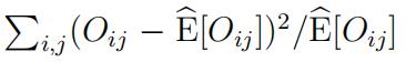
We define ‘close’ as having a small value of a quantity equal to or resembling (o − e)2, with o the observed values rij in each cell and e the premiums xiyj to be charged.
In insurance applications, the rule is that the deviation of o from its mean value will tend to be larger if this mean is large. So if we look at the unmodified sum-of-squares (o − e)2, the large values of o and e will have a large influence on the fitted values of xi and yj. Now assume that e is the mean value of o, and also a constant times its variance, such as when the observations are Poisson variables or multiples of those. Then if we look at (o − e)2/e instead, a scaled version of the sum-of-squares, all terms in the sum can be seen to have equal mean. See also MART, Ch. 9.3. Such quantities are known as chi-square statistics, and minimizing them to get estimates is called minimum chi-square estimation.
By asymptotic normality, the quantity approximately has a χ2
distribution, with as the number of degrees of freedom k the number of cells minus the number of parameters estimated.
The purpose of this assignment is to learn about
- using matrices, functions, iteration inR;
- usingthe optimization routines optim and optimize;
- improving a solution method by analyzing the first-orderconditions;
- fixed point algorithms; successive substitution.

1 Reading the data 计算机风险理论作业代写
Our data are average claims and the numbers of policies in a portfolio split up by gender, row-wise, and by three regions of residence, column-wise:
|
Gender |
Region 1
Policies Claims |
Region 2
Policies Claims |
Region 3
Policies Claims |
| 1 | 800 550 | 2400 364 | 1200 455 |
| 2 | 3200 625 | 1600 455 | 800 518 |
First we read the data and tell R to store them in 2 × 3 matrices:
n <- rbind(c(800, 2400, 1200),

c(3200, 1600, 800)) ## nr. of policies r <- rbind(c(550, 364, 455),

c(625, 455, 518)) ## average claim amounts
2 Using the general purpose routine optim()
Our first plan of action to find optimal premiums is simply to invoke R’s general purpose multivariate optimization routine optim(). The first argument of optim() is a vector of length equal to the number of parameters, and initially set to some starting values. Thesecond is a function to be minimized. Further and optional arguments might instruct optim to use a specific optimization technique or to stop only after many iterations.计算机风险理论作业代写
The first two elements of the parameter vector pars for the function dist1 defined belowrepresent x1, x2, the last three are y1, y2, y3. Using the fact that the outer product ˙x ⊗ ˙y is a matrix with (i, j) element xiyj, a straightforward function to compute the ‘distance’ d(˙x, ˙y) = (o − e)2/e is as follows:
dist1 <- function (pars) { x <- pars[1:2]
y <- pars[3:5]
f <- x o y ## o gives outer product sum(n * (r - f) ^ 2 / f) ## i.e., sum{(o-e)^2/e}
}
Note that oij here is actually nijrij, and eij is nijfij, which explains the n appearing in thenumerator for (o−e)2/e in the final line of the script. Since xiyj is to be used as a premium for cell (i, j), all parameters xi, yj must be positive. If the parameters are not constrainedto be positive, it is easy to see that the distance function has minimal value −∞, obtained when any f-value tends to −∞. Later on we will see some ways to find the solution we need, forcing optim to scan only the positive region.
We minimize this function dist1 by calling optim(), taking all starting values of the parameters equal to one.
By this choice, the initial fitted values are also all equal to 1, meaningwe start the search for the minimum in a point very far removed from the minimum when all parameters are positive. 计算机风险理论作业代写
oo <- optim(rep(1, 5), dist1)
| dist1(rep(1, 5)) | ## | 2,594,325,600 |
| oo$value | ## | 2554.5 |
| oo$convergence | ## | 1 |
| oo$counts | ## | 502 NA |
Instead of the outer product, we might have used for-loops the generate the matrix of cross- products xiyj. But unless the result in the next step of a for-loop depends on the result of the previous step(s), such as in recursive algorithms, it is better to use vector operationswhenever possible. First of all, they are easier to read, and second, they are very much faster.
The result of the optimization is a list of various fields, and we store it in object oo.
To see what these fields contain, do ?optim in R or in RStudio to access the help-file for optim. 计算机风险理论作业代写 From it, you learn that the par field of the object oo contains the optimal parameter values found, while oo$value gives the optimal function value. From the convergence field, you see that in spite of 502 function evaluations, convergence has not occurred. Possibly the fact that there are many equivalent solutions caused the problem with convergence. Indeed, any solution xi, yj is equivalent to αxi, yj/α, since they lead to the same fitted values xiyj, therefore to the same distance.
There are a number of ways to fix the problem of non-convergence:
- increase the number of function evaluations allowed (the default is about500);
- finda better starting value than taking all f[i, j] = xiyj values to be equal to 1;
- trya method of optimization other than optim’s default;
- usea method specific to this distance function (see Section 6).
Increasing the number of iterations 计算机风险理论作业代写
The iteration above stops after (about) 500 function evaluations. In the help-file ?optim you can see what to do to get more iterations. We increase the limit to 2000, and inspect the resulting object oo:
oo <- optim(rep(1, 5), dist1, control = list(maxit = 2000)) oo$value ## 2160.3
oo$convergence ## 0 oo$counts ## 530 NA
You see a 0 resulting for the convergence field, meaning convergence has occurred.
Verifying if the solution found is in fact optimal
In view of the difficulty we experienced in finding the best solution, caused in part becausewe started far from the minimum and close to the border of the feasible region, we are stillsuspicious of the outcome found. It may very well be that we have not landed in one ofthe global minima, but in a critical point that is in fact a saddle point.计算机风险理论作业代写
That means that though decrease is not possible by changing only one of the parameters, it might be that ifwe look in another direction, lower values of the objective function can be reached. To check if a critical point of a one-dimensional function is in fact a minimum, you look at the sign of the second derivative. In case of n-dimensional functions, to check if a solution to thenormal equations with ∇f (˙x) = (∂f /∂x1, . . . , ∂f/∂xn) = ˙0 is a minimum, you can look at the Hessian. The Hessian is the matrix ∇2f (˙x) of second partial derivatives. R gives us the possibility to calculate a numerical approximation to the Hessian after having run optim.
Consider the Taylor expansion (˙x, ˙y are arbitrary n-vectors; (·, ·) is the in-product):

Suppose ˙x is a critical point, so the gradient ∇f (˙x) = ˙0. If ∇2f (˙x) is not positive definite,there exists a vector ˙u with ˙uT∇2f (˙x)˙u < 0. Then f (˙x) cannot be minimal, because for a small enough real number η, taking ˙y = ˙x + η˙u we will have
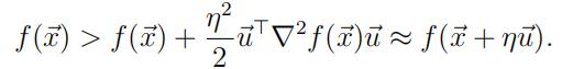
So for the critical point found to be a minimum, the Hessian must be positive definite.One way to check that is to find the eigenvalues of that matrix and verify that they are allpositive. We can run optimHess to find the approximate Hessian at the optimum found byoptim, or, like we do here, we can add an argument hessian=TRUE to make optim output this matrix in the field oo$hessian. To find its eigenvalues, we use eigen().
Consider the following script and its output reproduced in comments:
oo <- optim(rep(1, 5), dist1, hessian=TRUE, control = list(maxit=2000)) all(eigen(optimHess(oo$par, dist1))$values > 0) ## is FALSE
## Apparently the routine stopped with ‘convergence’ in a saddle point. oo <- optim(oo$par, dist1, hessian=TRUE, control = list(maxit=2000)) all(eigen(optimHess(oo$par, dist1))$values > 0) ## is now TRUE oo$value ## 2132.833
oo$convergence ## 0 oo$counts ## 164 NA 计算机风险理论作业代写
After the first call of optim, the approximate Hessian has negative eigenvalues, indicating that we ended up in a saddle point. When rerunning optim starting from the saddle point,we escape from this saddle point, which is possible because in its initial phase, optim takeslarger steps than in the end. Since all eigenvalues of the Hessian are now positive, we are no longer in a saddle point but in a minimum, although possibly only a local one.
Q1 Which elements of the Hessian of the function 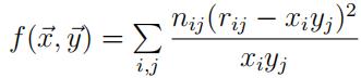 are zero?
Check with the values in the approximate Hessian in oo$hessian.
Improving the starting value 计算机风险理论作业代写
The interpretation of the parameters xi, yj above is that the observed average claims rij should be close to the fitted values xiyj. Since (x1, x2, y1, y2, y3) gives the same fitted values xiyj as (x1/x1, x2/x1, y1x1, y2x1, y3x1), we can set x1 = 1. Then x2 is the factor by whichclaims for gender 2 are larger or smaller than those for gender 1.
From the table in Section1 we see that average claims produced in cells of gender 1 total 550 + 364 + 455 = 1369; forgender 2 the total is 625 + 455 + 518 = 1598. The ratio x2 = 1.167 of these totals can be used as an estimate of the effect on the claims of being of gender 2 rather than 1.
In the same way we can find a crude estimate of the effect of being in region 2 rather than 1, which is (364 + 455)/(550 + 625) = 0.697. Similarly, the effect of region 3 instead of 1 is 0.828.计算机风险理论作业代写
With these ratios 1 : 1.167 for the rows and 1 : 0.697 : 0.828 for the columns,
we can ensure that our total fitted values x y are the same as the observed total values by multiplying all yj values by Σ rij/ Σ xiyj.
start.params <- 1
start.params[2] <- sum(r[2, ]) / sum(r[1, ]) ## effect of row 2 vs. row 1 start.params[3] <- 1
start.params[4] <- sum(r[ , 2]) / sum(r[ , 1]) ## effect of columns start.params[5] <- sum(r[ , 3]) / sum(r[ , 1]) ## 2 and 3 vs. column 1 start.params[3:5] <- start.params[3:5] * sum(r) /
sum(start.params[1:2] o start.params[3:5]) dist1(rep(1,5)) ## 2,594,325,600
dist1(start.params) ## 2,481.83
optim(start.params, dist1)$value ## minimum is now minus infinity
Starting from the naive initial estimates (1, 1, 1, 1, 1), the optim function converged to a saddlepoint, as you can see by running the scripts above. When starting from the more sophisticated starting values, at a distance one million times less than the naive values, the optim function steps out of the positive region and finds the global minimum.
Other methods for optim than the default one
The help-file for optim states that it is a general-purpose optimization based on Nelder-Mead, quasi-Newton and conjugate-gradient algorithms. It includes an option for box-constrained optimization and simulated annealing.
The following commands show the minima found by all available techniques on our problem.计算机风险理论作业代写
for (meth in c(“Nelder-Mead”, “BFGS”, “CG”, “L-BFGS-B”, “SANN”)) print(optim(rep(1, 5), dist1, method = meth,
control = list(maxit = 2000))$value) ## Nelder-Mead BFGS CG L-BFGS-B SANN
## 2160 -4e+35 -7e+36 2132.833 ~ -1e+13
As you can see, “L-BFGS-B” stumbles upon the minimum in the positive area. The default method “Nelder-Mead” gets stuck in a saddlepoint. The other methods “BFGS”, “CG” and “SANN” end up in the area with negative parameters and in fact are heading towards the correct global minimum −∞. Simulated ANNealing stops after a fixed number of function evaluations. Its outcome is stochastic; rerunning gives slightly different results.
3 Restricting the search for parameters to positive ones
Three ways to force optim to consider only positive parameter values are explored in the questions that follow:
- Imposebounds on the parameters in the optim function;
- For inadmissible parameter values, return +∞ as the functionvalue;
- Insteadof fitted values xiyj with xi > 0, yj > 0, use exi eyj with xi, yj
Imposing bounds on the parameters 计算机风险理论作业代写
To implement the first idea, we can use the optimization method “L-BFGS-B”, which allows imposing bounds on the region to be searched. This is achieved by adding named arguments lower = 1e-6, method = “L-BFGS-B” to the optim function call. Taking lower bound 0 might lead to problems because the dist1 function is undefined at the boundary. Leaving out the method argument here does no harm; optim knows to switch to its only method that allows bounds, and gives a warning.
Q2 Adjust the optim-call above in this way. What is the resulting optimal distance?
How many function evaluations are needed? What premium would a policyholder of gender 1 living inregion 3 have to pay? Also start from start.params. Do you get a different result?
The optimization method used in fact computes a finite-difference approximation to the gradient, that is, the vector of partial derivatives (∂d/∂x1, ∂d/∂x2, ∂d/∂y1, ∂d/∂y2, ∂d/∂y3), with d the function minimized. These partial derivatives are approximated using the formulaf j(x) = (f (x + h) − f (x − h))/2h for some small h. So each iteration step in fact requires 2p + 1 function evaluations, with p the number of parameters, but these extra steps are not included in the oo$counts field. 计算机风险理论作业代写
Q3 Recall Taylor expansions for real functions f at x + h and x − h:
f (x ± h) = f (x) ± hf j(x) + h2f jj(x)/2 + O(h3).
Here O(hk) is to be read as ‘terms of order hk and larger’ (big O notation), or equivalently, as ‘some power series in h with as first term an arbitrary constant times hk’.
Use these expansions to prove that for a finite-difference approximation with difference h to the derivative of f at x, the error is of order h2, that is,
f j(x) = f (x + h) − f (x − h) + O(h2).
2h
Assigning distance +∞ to inadmissible parameter values
Q4 Implementing the second idea in the beginning of this section, use a distance function dist2 that equals dist1 except for the last command. To ensure that the resulting parameter esti- mates are all positive, replace this line by ifelse(all(pars>0), sum(n*(f-r)^2/f), Inf).
For a quick check if your code is right, use the optimal parameter values to find out what premium a policyholder of gender 1 living in region 3 would have to pay.
Optimizing logs of parameter values
Q5 For the third method, write a distance function dist3 that equals dist1 but with the commands x <- pars[1:2] and y <- pars[3:5] replaced by x <- exp(pars[1:2]) and y <- exp(pars[3:5]).
Compare the distances between fitted values and observations as computed at start.paramsby dist1 and by dist3. If they are not the same, rethink your code.计算机风险理论作业代写
Minimize the distance starting from the naive starting values. Check convergence, and findthe resulting optimal distance and the number of function evaluations. If the resulting dis- tance is a lot more than the actual optimum, check your code. If it is rather close but not very close, try if running optim from the alleged optimum found gets you to the real optimum.
From the optimal parameter values, find what premium a policyholder of gender 1 living in region 3 would have to pay.
Does optimizing starting from start.params lead you to the actual optimum directly?
Using non-default methods for optim 计算机风险理论作业代写
The following script again runs all methods optim provides for our problem, but now with distance +∞ for infeasible parameters.
for (meth in c("Nelder-Mead", "BFGS", "CG", "L-BFGS-B", "SANN")) { with(optim(rep(1, 5), dist2, method = meth),

cat(value, "\t", counts, "\t", meth, "\n"))

}

##   Nelder-Mead BFGS CG L-BFGS-B SANN

## 502 NA 204  27 250  53 27  27 10000 NA

## 2554.523 2132.838 2132.833 2132.833  2136.305
Based on these results for our specific example, we cannot say we prefer one method over another. But in this case the default method Nelder-Mead is definitely worst.
The “BFGS”, “CG” and “L-BFGS-B” methods use finite-difference approximations to the gradient, counted in the second number in the $counts field.
Ordinary least squares 计算机风险理论作业代写
Now consider the ordinary (unweighted) least squares distance i,j (rij−xiyj)2 between fitted and observed average claims paid. We are going to use a call to optim with this distance.
Q6 Adapt the function dist2 into a function dist4 that produces the unweighted sum of squares distance. How much premium does a person of gender 1 in region 3 have to pay now? The optimal premiums should of course resemble the ones found with the weighted distance function; if not, check your code again.
4 Reducing the number of parameters 计算机风险理论作业代写
Since especially for “Nelder-Mead”, the number of iterations is a lot more than expected for such a very small problem, we look deeper. It is obvious that if we divide all xi by some number and multiply the yj by the same number, the same fitted values xiyj result. So the problem is over-parameterized; without the first parameter, we can test the same fitted values, in fact fixing x1 = 1 by dividing/multiplying the other parameters by x[1]. Instead of at a five-dimensional parameter space, we now look at only four parameters x2, y1, y2, y3. The five-parameter version of the problem has a lot of equivalent minima, which might make it tough for the optimization routine to determine when it can stop.
Q7
Use a distance function dist5 which is dist3 but with the commands x <- exp(pars[1:2])and y <- exp(pars[3:5]) replaced by x <- exp(c(0,pars[1])); y <- exp(pars[2:4]).
We want to start from the fitted values resulting from start.param. Construct a vector
˙h such that (1, h1, h2, h3, h4) gives the same fitted values as start.param. Verify that the distances dist3 and dist5 computed at these vectors coincide.
Compare the numbers of iterations in the four- and the five-dimensional parameter space. What premium would a policyholder of gender 1 living in region 3 have to pay?
5 A more specific solution using the normal equations 计算机风险理论作业代写
A specialized method employing the specific properties of the problem will prove to be more efficient, in this case reducing the parameter space scanned to a one-dimensional one.
Recall that the quantity to be minimized is
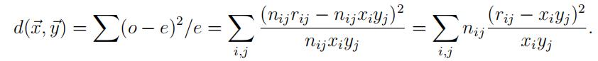
The first order conditions state that the gradient, that is, the vector of partial derivatives of d(x1, x2, y1, y2, y3), must be zero in the optimum. This leads to the normal equations. Solving these does not provide us with a full analytical solution to the problem, but the partial solution we get leads to a more efficient way to tackle the problem.
The partial derivative of d with respect to the parameter xt, t = 1, 2, is

Q8 Note that we do not look at ∂dibut at ∂d . Why?
And why is the second summation only over j?
Write down the partial derivative for xt if the dimension of the data arrays nijk and rijk is three and the fitted values are of the form xiyjzk.
So in the two-factor case, the normal equation ∂d/∂xi = 0 can be written as
The normal equations ∂d/∂yj = 0 are found analogously. Rearranging leads to the following system of equations in xi, yj, not having an analytical solution:
So if x1 = 1 and x2 is fixed, the optimal yj values are readily found from the second equation in (2). As a consequence, we only need to find the best x2. With only one parameter remaining to be determined, in our example this can be done using the one-dimensional minimization function optimize:
dist6 <- function(x2) { x <- c(1, x2)
y <- rep(1, 3) ## ‘declare’ array y before it can be used for (j in 1:3)
y[j] <- sqrt(sum(n[, j] * r[, j] ^ 2 / x) / sum(n[, j] * x)) ## eqn. (2b) f <- x o y
print(sum(n * (r - f) ^ 2 / f)) ## is also the result returned
}
(x2 <- optimize(dist6, c(.5, 2))$minimum)
## 11284 37767 106783 2643 2203 2134.6 2132.8 (5x)
## optimum 2132.833 found in 11 iterations; located at x2 = 1.181
Q9
Find the optimal yj values corresponding to ˙x = c(1, x2). What premium would a policy- holder of gender 1 living in region 3 have to pay? 计算机风险理论作业代写
The method used by optimize is a combination of golden section search and successive parabolic interpolation, and was designed for use with continuous functions. As one sees by inspecting the output, convergence in the optimize call is not monotone. Perhaps heway new candidates (˙x, ˙y) are determined by optimize can be improved upon. This will be explored in the next section.
6 Successive substitution; a fixed point algorithm
From the equations (2) derived above, we see how to find the optimal ˙y, given ˙x, by substi- tuting ˙x in the second equation. But this also works the other way around: with any vector ˙y, we can find the best ˙x = f (˙y). Following this through leads to an algorithm called ‘successive substitution’. It goes as follows:
1.Asa starting value for ˙x, take for instance xi = 1 ∀i; 计算机风险理论作业代写
2.Substitutethe latest ˙x to find a new ˙y = g(˙x) using the second equation in (2);
3.Substitutethe latest ˙y to find a new ˙x = f (˙y) using the first;
4.Iteratesteps 2 and 3 until ‘convergence’.
If h(˙x) d=ef f (g(˙x)) is continuous and the sequence ˙x → h(˙x) → h(h(˙x)) → · · · converges,
it must be to a point ˙x∗ having the property that ˙x∗ = h(˙x∗). Such a point is called a fixed point of the function h, hence the name ‘fixed point algorithm’.计算机风险理论作业代写
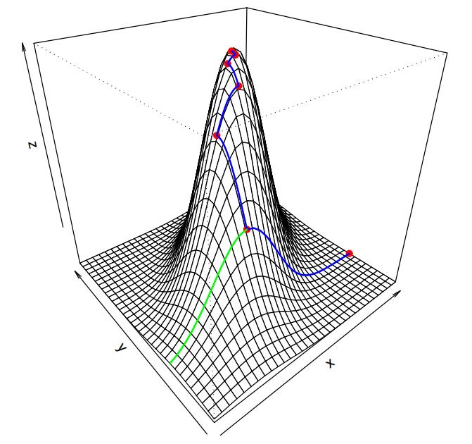
The figure below shows how this optimization method works in two dimensions. Starting at the rightmost dot in the picture, we maximize over x keeping y fixed. Next we keep x fixed and go toward the top by choosing the maximizing y. Then maximize for x keeping y fixed, and so on until we consider the top to be reached.
For the case at hand, the successive substitution method can be implemented as follows:
y <- rep(1, 3)
x <- rep(1, 2) dis <- 0 repeat {
olddis <- dis
for (j in 1:3)
y[j] <- sqrt(sum(n[, j] * r[, j] ^ 2 / x) / sum(n[, j] * x)) ## (2b) for (i in 1:2)
x[i] <- sqrt(sum(n[i, ] * r[i, ] ^ 2 / y) / sum(n[i, ] * y)) ## (2a) y <- y * x[1]
x <- x / x[1] ## normalize s.t. x[1] == 1 f <- x o y
dis <- sum(n * (r - f) ^ 2 / f)
print(dis) ## 6243 2225 2135 2132.879 2132.834 2132.833 (3x)
if (abs((dis - olddis)/dis) < 1e-8) ## the convergence criterion break
}
x[1]*y[3] ## 447.8525 is the estimated risk premium in cell (1,3)
This way, the optimum in seven digits is reached in six steps. Notice that by construction, the distances found decrease monotonically, and if the starting values are positive, there is no risk of trying to inspect inadmissible negative parameter values.计算机风险理论作业代写
Q10Would dis == olddis be a good convergence criterion? And how about 1e9 + dis == 1e9 + olddis?
Hint: what is the result of 1e9 + dis – 10^-(6:9) == 1e9 + dis + 10^-(6:9)?
Some remarks:
- We aggregated our data on the individual policies by two risk factors Every additional risk factor adds an extra dimension to our data array, see Q8. Also,every
additional risk class like a third gender or a fourth region means an extra parameter. So reverting to successive substitution might very well be necessary to prevent long waits.
- Take a closer look at the fit results. To compare the fitted values f with r,do:
round(f / r, 3)
## 0.969 1.026 0.984 计算机风险理论作业代写
## 1.007 0.970 1.021
In this example, the best fitted values f are rather close to the observed values r. So the model explaining the number of claims in a cell as a product of a gender effect and anindependently operating region effect is quite satisfactory in this case. As one sees fromf/r, the gender effect in all regions is about the same. This means that there is hardly any interaction between these risk factors. A statistical test for this situation would not lead to rejection of this model in favor of one having gender effects that differ by region, in fact having six parameters; the distance between fitted and observed values is not so big. See MART, Ch. 9.
-
Thesolution of the successive substitution method cannot be improved by taking other row coefficients, keeping the column coefficients fixed, or vice But as explained
earlier, it might be that we land in a saddle point, and can improve the solution by changing both. Even if this is not the case we may end up in a local minimum, missing a global minimum elsewhere in the feasible region. 计算机风险理论作业代写
The fitting method above, known in actuarial literature as the Bailey-Simon (BS) method, has a nice property. By minimizing the chi-square statistic, fitted values are found with the property that at group level, the total of the fitted values is at least the total of the observed ones. For a proof of this statement see MART, Property 9.3.7. To show that our example, in any case, does not provide a counterexample of this property, for both possible margins (1 = rows, first index, 2 = columns) of the matrix of differences (f-r)*n we apply the sum function to get row sums and column sums. One may also use the functions rowSums and colSums, faster for large matrices; mind the capitalization.
apply((f – r) * n, 1, sum) ## 579 488
apply((f – r) * n, 2, sum) ## 268 640 159
Q11
All the signs are positive, so perhaps not for each cell, but in any case for each group men/women and regions 1/2/3, the projected average claims is at least the observed average claims. The actuary may rest comfortably; the premiums found are ‘prudent’.
Instead of the Bailey-Simon normal equations (1) that lead to row and column sums offitted values larger than those for observations, we want to find xi, yj values such that these marginal totals match exactly, therefore
Σ nij rij = Σ nij xi yj and Σ nij rij = Σ nij xi yj. (3) 计算机风险理论作业代写
Rewrite these equations in such a way that they allow the technique of successive substitution to be used, cf. (2). Having saved the BS fitted values for later use by f.BS <- f, find the optimal xi, yj values as above. Iterate until the maximal absolute value of the row and columns sums of (r – f) * n / sum(n * r) is less than 1e-10.
Check if the marginal totals fitted and observed agree, and find the premium for a person of gender 1 living in region 3.
Also check the total Bailey-Simon premiums asked per cell and compare with the ones with fitted marginal totals.
Compare the total premiums paid when estimated by BS to the one computed from fitting marginal totals, and also to the total claims actually paid.
7 Successive substitution on a larger portfolio
In the previous sections, we have found a method to fit multiplicative premiums for a small example portfolio classified by two factors, with 2 and 3 levels. The premiums were con- structed so as to minimize a chi-square distance (Bailey-Simon), or in such a way that the marginal totals of fitted and observed values agree. To show how efficient this method canbe, we consider in this section a simulated artificial portfolio of 299561 car insurance risksgenerating 29645 claims in a particular year.
The policies are divided into 500 rows and 40columns.
A different row number might mean a different combination of risk characteristicsreflecting driver quality, such as claims history, age and profession of the driver, weight andprice of the car, mileage, region of residence and many more. A different column might mean different policy characteristics such as which events are actually covered, deductible, and more. But what they represent is not really important here.
The data mij are the numbers of claims made by the nij drivers with factor 1 at level i, factor 2 at level j, and they are assumed to be Poisson(nijxiyj) distributed and independent. The nij, xi and yj values also resulted from random drawings and are assumed given. All cells are non-empty by construction, avoiding problems because 0/0 is undefined (NaN, not a number).计算机风险理论作业代写
This is how to reconstruct the data:
set.seed(3) n.row <- 500
n.col <- 40 xx <- sample(10:30, n.row, repl = TRUE) / 20 ## between 0.5 and 1.5 yy <- sample(30:70, n.col, repl = TRUE) / 500 ## between 0.06 and 0.14 n <- matrix(sample(5:25, n.row * n.col, repl = TRUE), n.row, n.col) ## 5 .. 25 m <- rpois(n.row * n.col, (xx o yy) * n) m <- matrix(m, n.row, n.col) r <- m / n cat(sum(m), "claims by", sum(n), "policies\n")
It can be shown that the normal equations that the maximum likelihood estimates of xi, yj must satisfy are precisely the marginal totals equations (3). The purpose of this section is to compare the performance of the successive substitution method discussed above andthe standard algorithm to maximize the likelihood for this problem. Because it is a special case of a so-called generalized linear model, it can be solved by a method called iteratively reweighted least squares (IWLS). The generalizations of the multiple regression model of the econometrics courses are that we have here Poisson distributed dependent variables, a multiplicative model for the means and categorical explanatory variables, rather than normally distributed homoskedastic observations and an additive model such as in the ordinary linear model.计算机风险理论作业代写
The built-in glm routine in R requires that the data are stored in a vector, not a matrix.
Also, the explanatory variables row and column number are categorical values, meaning that they are to be treated ‘as factor’. The final command below performs the maximum likelihood estimation of our model. The result of the fitting of the model is stored in glm.result, taking up 94 Mb of memory on a 64-bit system. The time spent by this system on the glm call is about 40 seconds. Note that the likelihood function is a function of 540 parameters and 20000 data points, so it is not surprising that maximizing it takes a while.
m.vec <- as.vector(m) n.vec  <-   as.vector(n) i.vec <- as.factor(row(m))

j.vec <- as.factor(col(m))

system.time({

glm.result <- glm(m.vec ~ i.vec + j.vec, poisson, offset = log(n.vec))

})
Q12 计算机风险理论作业代写
Now apply successive substitution to find estimates for the xi and yj parameters that are a solution to the system (3), involving 540 equations in as many unknowns. Use the same stopping criterion as in the previous question, except now with tolerance 1e-14. You will notice that convergence still only takes a handful of iterations. Use the system.time function to find the time spent on the successive substitution.
By executing range(fitted(glm.result) – f*n), verify if the solutions found by both methods are the same in about 8 decimal places. If they are not, check your code.
So the specialized method spectacularly outperforms the standard solution in this case, finding the same fitted values about a thousand times faster.

其他代写:代写CS C++代写 java代写 matlab代写 web代写 app代写 物理代写 数学代写 考试助攻 paper代写 r代写 金融经济统计代写 代写CS作业
