computer class Risk代写 assignment代写 likelihood estimates代写

Assignment computer class Risk Theory 2017–2018; week 3

computer class Risk代写 determining maximum likelihood estimates for parameters;•Makeham’s and Gompertz’ mortality laws;mortality rates;

The purpose of this assignment is to learn about  computer class Risk代写

• determining maximum likelihood estimates forparameters;
• Makeham’s and Gompertz’ mortalitylaws;
• mortalityrates;
• findingmean remaining lifetimes by estimating them from the sample or computing them from the cdfs using the maximum likelihood estimates of the parameters;
• proportional hazardmodels;
• the Akaike Information Criterion(AIC); computer class Risk代写
• making appropriate

Makeham’s and Gompertz’ mortality laws computer class Risk代写

In the year 1899, 100 000 people were born in the Netherlands. Their exact age-at-death X_i (in fractional years) was not recorded, only its integer part K_i = |X_i∫, i = 1, . . . , 100 000. All their realized ages-at-death k₁, . . . , k₁₀₀₀₀₀ (integer) are known by now. They are summarized

in a table with the numbers of people d_x that died at a particular age x = 0, 1, . . . 

This tableof the ‘curtate lifetimes’ can be read in (in R) as follows:

rm(list = ls(all = TRUE))

d.x <- scan(n = 95) ## numbers that died at age x = 0,1,2,...

2618	390	85	41	26	26	30	32	34	33	22	37	28	32	25
20	36	38	29	27	30	38	28	38	52	33	48	49	45	48
51	55	56	55	67	76	82	104	92	114	94	121	139	152	163
205	196	237	275	296	343	382	421	526	582	622	742	878	921	1075
1216	1398	1594	1840	1923	2253	2483	2688	3186	3346	3710	3817	4121	4490	4688
4734	4864	4884	4756	4560	4120	3740	3385	2756	2079	1563	1086	727	455	228
103	42	17	7	1

These figures are the numbers d_x of indices i = 1, . . . , 100 000 for which k_i = x, x = 0, . . . , 94.Wedon’t need the full sample k₁, k₂, . . . ; the frequencies D_x are sufficient statistics, because they correspond one-to-one with the ordered sample K₍₁₎, K₍₂₎, . . . Exactly for which i we have K_i = x does not give us information about the parameters of the lifetime distribution, only the number of times d_x this occurs.computer class Risk代写

Q₁ Using the rep() function, reconstruct the sorted sample from the frequencies in d.x. computer class Risk代写

Note that in this assignment, we use a simpler model than is used in most population studies.In the databases used, for a series of calendar years indexed t it is recorded how many people died at ages x = 0, 1, . . . . Also, the total number of days each person has lived having age x is totaled, and divided by 365 or 366. So dates of death and birth are incorporated. A person with x + 1^st birthday in calendar year t contributes 0 or 1 to the number of deaths at age x in year t, or to the one with age x + 1, depending on if he dies before or after his birthday.

He contributes the fraction computer class Risk代写

of the year he was alive having age x and age x + 1 to the total exposures of people of these ages in year t. In this assignment, we only know year of birth (1899) and age at death x = 0, 1, . . . . A person dying at age 65 may have died in calendar year 1964, after his birthday, or in 1965 before his birthday.

We can compute sample estimates of the probabilities of dying at age x for our group of 1899-born people, by dividing the number d_x of deaths at age x by the number of people n_x surviving up to age x. So we  want  to construct the vector n_x, using the values  of d_x,     x = 0, 1, . . . Note that we disregard migration into and out of the population.computer class Risk代写

As an example, consider a vector d_x = (1, 2, 3, 4, 5) with corresponding n_x = (15, 14, 12, 9, 5), stored in d.x and n.x. Not quite correct is sum(d.x) – cumsum(d.x); the result of that is (14, 12, 9, 5, 0). Less messy than manually adding 15 at the start of that vector and deletingthe 0 at the end is to start at the end of d.x and work backwards (using the rev() function, to reverse a vector, before and after).

Q₂ So what is a correct way to use the function cumsum() for this purpose? Fill in the dots below,

and check the last few entries of the estimated probabilities of dying stored in fr:

n.x <- ... 

head(n.x); tail(n.x) 

fr <- d.x / n.x tail(fr)

1 Makeham’s mortality law computer class Risk代写

The observations d₀, d₁, d₂ (and quite possibly d₃) can be seen to follow a different patternthan the remaining data. About 3% of the newborns die while still infants. For the remaining 97%, the ages-at-death are assumed to have arisen from a continuous lifetime distribution function called Makeham’s Law; see also exer. 3.9.16 in MART.

The mortality rate of a continuous random variable X denoting a life-time is defined as

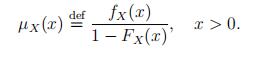
(1)

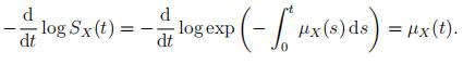
By the chain rule, we also have

                     (2)

Life-time X has a Makeham(a, b, c) distribution if µ_X(x) = a + bc^x for parameters a, b > 0,

c > 1. Gompertz’ law is the special case with a = 0.

The mortality rate can be found from the cdf, see (2). The opposite is also true. The survival probability S_X(t) = 1 − F_X(t) can be deduced from a mortality rate µ_X(·) using

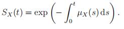                   (3)

To show that log S_X(t) equals the integral in the rhs, observe that log S_X(0) = log 1 = 0 and

To find S_X(x) = Pr[X > x] for the Makeham and Gompertz distributions, for which µ_X(x) =a + bc^x, note that by  (2) we  have  − log(S_X(x)) = ax +   ^b  c^x + C  for some constant C. The value of C can be deduced from S_X(0) = 1, and we get

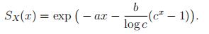
(4)

Some remarks on mortality rates/laws: computer class Risk代写

• Themortality rate, aka the failure rate, characterizes a life-time distribution just like the density or the
• µ_X(x) dx = 1−FX (x) can be interpreted as the conditional probability of deathbetween x and x + dx for someone alive at age x.
• IfX = min{Y, Z} and Y, Z are independent, then 1 − F_X(x) = Pr[Z > x] Pr[Y > x], hence µ_X(x) = µ_Y (x) + µ_Z(x).
• Sowhile using mgf/cgf/cf/pgf is convenient when looking at the sum of independent r.v.’s, consider using the mortality rate transform when looking at their minimum.
• Makeham’s mortality lawµ_X(x) = a + bc^x arises from a competing risks model, since people die from whichever happens first:
  • ‘accident’ at age Z ∼ exponential(a) (note that µ_Z(x) ≡ a, as is easily proved),or
  • ‘senescence’ at age Y ∼ Gompertz(b,c).computer class Risk代写

We can prove that a Gompertz random variable equals a transformed exponential random variable. To be precise, if V ∼ exponential(1) then

To  prove that, note that we have Pr[V  > v] = e^−v, and c^Y  − 1 = . Then

so Y ∼ Gompertz(b, c); see (4) with a = 0.

We can easily write functions rGompertz to generate random deviates from the Gompertz distribution, as well as rMakeham to draw a sample from a Makeham distribution. We first draw a sample from the senescence distribution, by transforming an exponential random variable,

and next use the pmin (parallel minimum) function, as follows:

rGompertz <- function(n,b,c) log(1+rexp(n)*log(c)/b)/log(c) rMakeham <- function(n,a,b,c) pmin(rGompertz(n,b,c), rexp(n)/a) a <- 5e-4; b <- 8e-5; c <- 1.09; n <- 2000

set.seed(2525); G <- rGompertz(n, b, c)

set.seed(2525); M <- rMakeham(n, a, b, c) ## same Gompertz dying ages rbind(Gompertz=summary(G), Makeham=summary(M))

## Min. 1st Qu. Median Mean 3rd Qu. Max. ## Gompertz 4.8480 67.15 77.33 74.51 85.01 105.5

## Makeham 0.2809 65.54 76.47 72.92 84.68 105.5

A minimal R-function (no parameter checks) to compute the survival function (4) for the Makeham and Gompertz probability laws, with parameters a ≥ 0, b ≥ 0, c > 1, is as follows:computer class Risk代写

sMakeham <- function (x, a, b, c) ifelse(x<0, 1, exp(-a*x-b/log(c)*(c^x-1)))

Q₃ Write an R-function computer class Risk代写

to compute the probability of having curtate lifetime k = 0, 1, . . . , that is, Pr[K  = k] = Pr  X ∈ [k, k + 1)  = Pr[X  ≥ k] − Pr[X  ≥ k + 1], where K  = |X∫. When k is not integer, that is, k > |k∫, the probability Pr[K = k] should be zero.

Note that because S and F are continuous, Pr[X ≥ k] = Pr[X > k] = S(k). Now using

sMakeham defined above, fill in the dots to get the discrete density:

dMakeham <- function (k, a, b, c) ifelse(k>floor(k), 0,

(sMakeham(...)-...))

For ages x = 0, 1, 2, 3, 4, 7, 10, 30, 50, 70, 90, compare actual and expected numbers of people born in 1899 and dying at age x. Use parameters a <- 3e-4; b <- 3e-6; c <- 1.15.

Hint: Define x <- c(0:4,7,10,30,50,70,90). We want to compare the observed numbers d.x[x+1] with the expected numbers. To compute expected numbers, keep in mind that the number of people who die at age x is a binomial random variable with parameters . . .

Graphically illustrating the data computer class Risk代写

First we make a plot, of histogram type, of the table of lifetimes. Note that rounded-down ages-at-death start at 0, but indices of vectors in R start at 1:

ages <- 0:(length(d.x)-1) 

plot(ages, d.x[ages+1], type="h")

Because of infant mortality, the first few counts are special. In fact the lifetimes arose from a mixed distribution, with early deaths mostly caused by infant mortality, later ones obeying Makeham’s Law. To get estimates for the a, b, c parameters, one might replace the first few data points by fake ones following the pattern of the others. More correct is to simply ignore d₀, d₁ and d₂ for the parameter estimation, considering only a subset of the ages x.computer class Risk代写

allages <- ages; ages <- 3:max(ages)

 plot(ages, d.x[ages+1], type="h")

This plot looks very smooth. And it should, because our data are not real data, but a large sample of random drawings from an actual Makeham cdf (except for infant mortality), see above.

2 The likelihood of the Makeham parameters computer class Risk代写

The likelihood of parameters is the probability under these parameters of a random sample K₁ = k₁, K₂ = k₂, . . . , K_100 000 = k_100 000, with K_i = |X_i∫, therefore

We will throw out the sample elements with k_i < 3, to be blamed on infant mortality rather than influenced by the Makeham parameters.

Q₄ Verify that the negative

of the logarithm of the likelihood is computed by the function loglikMakeham that follows. In this function, abc is a vector of length 3 with values for a, b, c, and ages is a vector of numbers containing the subset of {0, 1, . . . } of the ages considered.

loglikMakeham <- function (abc) ## function to be fed to optim()

{-sum(log(dMakeham(ages, abc[1], abc[2], abc[3])) * d.x[ages+1])}

We compute the negative of the loglikelihood to get positive numbers. This has the benefit that we avoid having to specify that the optimizing function should maximize rather than minimize. The help-file ?optim states: “By default optim performs minimization, but it will maximize if control$fnscale is negative”.computer class Risk代写

Next, we find ML estimates of a, b, c on the basis of this sample, using the optim() function:

start <- c(1.5e-4,2e-4,1.1)

oo <- optim(start,loglikMakeham); oo

a.hat <- oo$par[1]; b.hat <- oo$par[2]; c.hat <- oo$par[3]

The starting values (we took a = 0.00015, b = 0.0002, c = 1.1) should be in the feasible region. They have been chosen in the vicinity of Makeham parameters found in the literature. If problems arise for other samples, try different starting values. Note that computing sMakeham might easily give numerical difficulties at high ages.computer class Risk代写

This optimization goes rather fast. If we would have been working with the full sample of size 100 000 instead of the condensed frequency table, however, it would have taken longer. Even though having to do a few hundred iterations seems a lot, we are not going to look into how it may be improved. Running warnings() we see that often parameter vectors were tried leading to not computable Makeham log-densities (NaN = not a number).computer class Risk代写

3 Mortality rate

For lifetimes and other ‘failure times’, one is often interested in the probability of dying in the next time period of length h, conditionally given survival up to age t:

Note that µ_X(t) = − d log S_X(t) is the mortality rate, see (2).computer class Risk代写

In the Makeham case, S_X(t) is as in (4); the mortality rate is µ_X(t) = − d log S_X(t) = a+bc^t.

Taking h = 1 year, we can compute sample estimates of these failure rates, by dividing the number d_x of deaths at age x by the number of people n_x surviving up to age x. So we need the vector n_x as constructed before using the values of d_x, x = 0, 1, . . .

Except at the start and at the end, the observed mortality rates closely follow the estimated ones. See the plot resulting from:

plot(allages,fr,type="l") 

lines(allages,a.hat+b.hat*c.hat^allages,col="green")

The failure rate is actually a conditional probability of dying the next instant given alive. computer class Risk代写The Makeham density is the unconditional equivalent. The fitted Makeham density can thus be compared to the number of people dying at ages 0, 1, . . . , resulting in:

y <- d.x/sum(d.x) plot(allages,y,type="h",col="blue")

lines(allages, dMakeham(allages,a.hat,b.hat,c.hat), col="red")

After infant mortality, Makeham’s Law fits the data well.computer class Risk代写

4 Average age-at-death; number  of retirement  years

To compute the average age-at-death, compute the observed sample mean. For the people dying  according  to  Makeham’s  Law  with  parameters  aˆ, ˆb, cˆ,  the  expected  value  equals,  cf. MART (1.33):

To reconstruct the sample mean, we use the function sum(), accounting for frequencies. For the ML-estimated expected value, we use integrate():

sum((allages+0.5) * d.x) / sum(d.x) ## 69.85531

integrate(sMakeham, 0, Inf, a.hat,b.hat,c.hat) ## 72.04979 +/- 0.00099

Q₅ Explain why allages+0.5

is used rather than just allages. Also, indicate why these out- comes are so different, and what should be done to get outcomes that are closer.computer class Risk代写

Q₆ Also relevant is the mean number of pension years after age 65 for people born in 1899. Give both the direct sample estimate and the value resulting from integrating the tail of the ML- estimated survival function. Compute both the mean number of pension years a newborn in 1899 enjoyed and the mean number for those born in 1899 and surviving up to age 65.

5 Proportional hazard models 

It is sometimes claimed that because of smoking, mortality rates are multiplied by a certain factor, let’s say, doubled. Under Makeham’s law, a person has mortality rate a + bc^x, so doubling this rate simply means replacing a by 2a, b by 2b. We want to investigate what effect doubling the mortality rate has on the full life expectancy.

Q₇ The hazard rate with failure time

(age-at-death) X is called the mortality rate (2) in life insurance. What is the hazard rate in case of an exponential(λ) failure time? How does doubling this rate affect the mean failure time?

If X, Y are independent, their joint survival function is S_min{X,Y }(t) = Pr[X > t, Y > t] = S_X(t)S_Y (t). Therefore, from (2), µ_min{X,Y }(t) = µ_X(t) + µ_Y (t), so if X ∼ Y , then min{X, Y } has twice the hazard rate of X. This gives a natural interpretation for replacing a mortality rate by any integer multiple of it, but in fact these rates can be multiplied by any positive real and still give a valid mortality rate function.computer class Risk代写

Q₈ For a survival function S(t),computer class Risk代写

what is the resulting survival function S_f (t) if the mortality rate is multiplied by some f > 0? Is it a proper survival function, that is, continuously decreasing from 1 at 0 to 0 at ∞?

Q₉ Using the integrate function as above, and parameters a <- 2.2e-4; b <- 2.7e-6; c

<-  1.124, compute the mean age-at-death if the mortality rate is multiplied by  a factor    f = 2^k, k = −3, . . . , +3. Plot the mean age-at-death against k, and conclude that the mean age-at-death is very nearly log-linear in the proportionality factor.

With these parameters for a Makeham law, what is approximately the effect of doubling the mortality rate on the mean age-at-death?

6 Reducing Makeham’s law to Gompertz’ computer class Risk代写

Q10 Gompertz’ law is Makeham’s but with a = 0. Find ML estimates for this subfamily of functions, plot the result and compare with the fit by Makeham. Use the AIC 2k − 2A, where k is the number of parameters in the statistical model and A is the maximized value of the loglikelihood function for the estimated model.

更多其他：考试助攻 代写作业 加拿大代写 北美cs代写 代写CS 统计代写 经济代写 计算机代写 物理代写 code代写 算法代写 计算机代写 

合作平台：天才代写 幽灵代写 写手招聘 Essay代写