
The Bartlett School of Environment, Energy and Resource
Energy Data Analysis代写 By submitting this document, you are agreeing to the Statement of Authorship:We certify that the attached coursework

MSc ESDA Coursework Title Page
UCL Candidate Code: Team R2-D2 (ZYHY9, BTPC2, BMKL5)
Module Code: BENV0091
Module Title: Energy Data Analysis
Coursework Title: Assessing Prediction Methods and Environmental Factors for Solar PV Generation
Module Leader: Dr Aidan O’Sullivan Energy Data Analysis代写
Date: 14.01.2019
Word Count: 4978 (from Title to end of Discussion including all figure titles & tables)
By submitting this document, you are agreeing to the Statement of Authorship: Energy Data Analysis代写
We certify that the attached coursework exercise has been completed by me/us and that each and every quotation, diagram or other piece of exposition which is copied from or based upon the work of other has its source clearly acknowledged in the text at the place where it appears.
We certify that all field work and/or laboratory work has been carried out by me/us with no more assistance from the members of the department than has been specified.Energy Data Analysis代写
We certify that all additional assistance which I/we have received is indicated and referenced in the report.
Please note that penalties will be applied to coursework which is submitted late or which exceeds the maximum word count. Information about penalties can be found in the MSc ESDA Course Handbook which is available on Moodle:
- Penalties for late submission:https://moodle-1819.ucl.ac.uk/course/view.php?id=9967§ion=30
- Penalties for going over the word count:https://moodle-1819.ucl.ac.uk/course/view.php?id=9967§ion=30
In the case of coursework that is submitted late and is also over length, then the greater of the two penalties shall apply. This includes research projects, dissertations and final reports.
Table of Contents Energy Data Analysis代写
Introduction 4
Existing Research 6
Methodology 8
Model Accuracy 9
Results 12
Training and test data 16
Linear model results (with and without penalisation term) 17
ANN Results 19
SVR Results 19
All Results 20
Discussion and conclusions 21Energy Data Analysis代写
References 23
Supplementary material 26
Table of Figures
Figure 1: SunLab Faro, Portugal, image by EDP Figure 2: Process for data analysis in this essay. Figure 3. Illustration of model structure
Figure 4: Daily total solar PV power output over four years with detail view
Figure 5: Generation with precipitation and atmospheric pressure, instantaneous readings Figure 6: Module A with horizontal, vertical and optimal generation by month
Figure 7: Comparison of Module A and Module B generation by month
Figure 8: The optional power generation, voltage generation and current generation by hour Energy Data Analysis代写
Figure 9: The power generation, voltage and current by month for Panel A in ‘Optimal’ orientation Figure 10: Power generation by ambient temperature and global radiation
Figure 11: Power generation by diffuse radiation and ultraviolet Figure 12: Power generation by wind velocity and direction
Figure 13: Power generation by precipitation and atmospheric pressure
Figure 14: Correlation matrix (left) without function fitting and (right) with transformed independent variables Figure 15: Coefficients function with L1 norm and log Lambda
Figure 16: Mean squared error to calculate an optimal lambda term in penalised regression Figure 17: Neural network generation predictions shown against actual generationEnergy Data Analysis代写
Figure 18: Support Vector Regression results plotted against actual generation Figure 19: All methods using weather variables inputs plotted over actual generation.
Table 1: Coefficient for each variable in linear regression model without penalisation term Table 2: R squared and adjusted R squared of linear regression model without penalisation term
Table 3: Coefficients for each variable in the ridge penalised linear regression for min method (left) and one standard error method (right)
Table 4: Results of different methods comparing R-squared and MAPE error metrics
Assessing Prediction Methods and Environmental Factors for Solar PV Generation
Introduction Energy Data Analysis代写
Solar photovoltaic (PV) panels have seen large growth in deployment worldwide and are expected to make up an increasing proportion of electricity generation. This increase brings a challenge to grid operators, utilities and policymakers due to the uncertainty and variability of generation output (Shang and Wei, 2018). PV power output varies significantly with solar irradiance and weather conditions. Daily, seasonal and locational variance, as well as project-specific factors like panel orientation, angle, and module technology also affect output. Accurate forecasting of the output of PV systems is vital for electricity grid balancing; load scheduling; procurement of ancillary or standby capacity; and for systems planning (Abuella and Chowdhury, 2015; Inman et al., 2013).
The output of solar PV has stochastic and seasonal character which varies with solar irradiance and weather conditions. More accurate predictions could reduce the need for standby or back-up generation (Nageem, R. and R, J. 2017) and lower system costs, as well as providing more accurate output forecasts for PV projects which are required for feasibility assessments.Energy Data Analysis代写
Power grids are designed to integrate particular amounts of energy from solar panels,
so predicting solar output will assist utilities to estimate the intermittent power in the grid, the stability of the grid and optimisations for trading in the electricity market (Nageem, R. and R, J. 2017). Predicting output from solar PV is recognised as an important way to meet the issues of stability, reliability, and balance of the power network (S. Sobri et al., 2018).Energy Data Analysis代写
There is a growing body of literature on various methods of solar PV generation forecasting in terms of characteristic and performance. This researches has established and examined different methods and models with useful findings about forecasting techniques. This paper aims to predict the power generation of solar modules using several forecasting methods and compare their effectiveness.
Weather features are highly localised, so any algorithmic approach should be able to generalise taking into account regional differences in weather patterns. In practice, generation forecasts are made using weather forecasts and therefore depend on their accuracy. We discuss the suitability of our approach over different PV projects and with varying data availability. This essay is accompanied by an online interactive display of different model predictions for SunLab Faro PV output, shown against actual generation and available here: https://esda.shinyapps.io/pv_app/.
Existing ResearchEnergy Data Analysis代写
Research into solar irradiance and solar power generation forecast has a long history starting in the early 20th-century (Marvin and Kimball, 1926). Today, attention has focused on the different instruments available for measuring the solar and wind power generation in advance. For example, number of searches in Google Scholar for solar irradiance and PV power forecasting reached 6340 queries (Yang et al., 2018). Yang et al. (2018) have done significant work on how to handle and review abundant literature on this topic using text mining; however this review of existing works has been carried out in the traditional manner.Energy Data Analysis代写
Quantitative knowledge of solar characteristics is crucial for performing solar energy in photovoltaic system as quantity of generated electricity is equivalent to solar radiation received on the PV. Quantitative methods offer an effective two methods for solar radiation prediction: the deterministic, which was used to model daily and hourly solar radiation (Liu and Jordan, 1960) and for estimating hourly diffuse irradiation from hourly global irradiation(Spencer, 1982); data-driven that use self-computing algorithm instead of complex mathematical equation and do no require information on solar dynamics (Deo and Şahin, 2017).
One of the most well-known and well-accepted reviews of solar forecasting methods was conducted by Inman at al. (2013).
This paper reviewed the theoretical basis of forecasting methods and classified them into five groups: artificial intelligence and stochastic, wireless sensor networks, satellite imaging, numerical weather predictions, and total sky imaging. According to Inman at al. (2013) regression methods and Artificial Neural Networks (ANN) perform well in both data-poor and data-rich environments; ANNs function as non-linear approximators for drawing good solutions for several multivariate non-linear and stochastic problems. Another important finding was that hybrid methods combining several techniques benefit over traditional approaches.Energy Data Analysis代写
For example, integration of numerical weather prediction (NWP) and satellite models with stochastic methods results in high accurate prediction for some time horizons. Ji and Chee (2011) in their work on predicting hourly solar radiation used a another hybrid approach combining Autoregressive and Moving Average (ARMA) to predict linear components and Time Delay Neural Network (TDNN) to predict the non-linear components. The paper supports the previous view on advantages of hybrid models over traditional techniques. Similarly, In 2012 Mandal et al. undertook a hybrid approach combining wavelet transform (WT) and artificial intelligence (AI) techniques to predict solar output based on solar irradiance and temperature data. This was evaluated as a highly accurate, efficient method which performs well in different seasons.
Forecasting tools can be divided into indirect and direct approaches.
In an indirect approach solar irradiance is forecasted with ANNs, SVM, time series models and others followed by usage of obtained data as inputs in commercial simulation software. Direct approaches aim to predict directly from readily accessible data (Wang, Su and Shu, 2016). This paper uses a partial functional linear regression model (PFLRM) for predicting daily PV output. This paper suggests a contrary view using intra-day time-varying pattern of solar data than the aggregated mean daily data.Energy Data Analysis代写
ANNs are currently the most popular method for making solar predictions (Antonanzas et al., 2016). In their review of papers on ANN as a solar irradiance prediction tool Qazi et al. (2015) have identified that ANN predictions are more accurate than statistical, linear, non-linear methods and concluded that neural networks increase the accuracy of monthly and hourly predictions.
Nageem, R. and R, J. (2017) have set up a new approach for output prediction from solar panels. Support Vector Regression (SVR) models, considered as statistical approach were used and compared with an analytical approach. Mean Absolute Percentage Error (MAPE) and Mean Absolute Error (MAE) was used to evaluate models. Using multi-input SVRs researchers found that changes in climate can significantly affect results; predictions obtained with current weather conditions demonstrated 36% error in power predictions over the following four hours. Error was also found to be high for analytical methods.Energy Data Analysis代写
More recent studies with improved versions of SVRs has been demonstrated by Shang and Wei, (2018).
Data for a proposed prediction model was taken in Arizona and Colorado, USA. Shang and Wei (2018) presented a prediction model based on a feature selection algorithm based on a hybrid forecast engine with support vector regression and enhanced empirical model decomposition (EEDM). The key aspects of this work can be listed as follows: EEMD generated small scale sub-signals from the solar signal to get more accurate predictions; the best input candidate was selected and transferred to the forecast engine for speed and accuracy optimization; SVM based hybrid forecast coupled with an intelligent algorithm implemented to improve accuracy; and finally, a new optimization algorithm to optimize the prediction process.
In the following sections will will present data gathering and preparation steps, followed by definitions of model accuracy metrics and characteristics of statistical methods employed. The final sections will show results obtained from different methods followed by our conclusions, discussion of shortcomings and potential future work.Energy Data Analysis代写
Methodology Energy Data Analysis代写
Data was obtained from SunLab Faro (EDP, 2019) as shown in Figure 1, a single solar PV installation consisting of six panel modules, three panels each from manufacturer ‘A’ and ‘B’, oriented horizontally, vertically and ‘optimally’ with rated power output of 220 Wpeak (see supplementary material for datasheets). The SunLab project is owned by EDP, a global energy company, with the stated aims of assessing performance, reliability, new technologies, optimisation and the development of analytical tools including forecasting.
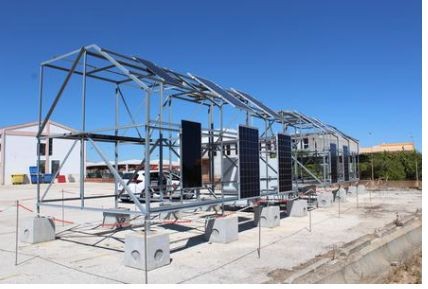
Figure 1: SunLab Faro, Portugal, image by EDP
SunLab uses various PV modules in different conditions and orientations,
over four locations across Portugal’s western coastline. Power, current, voltage, and module temperature are available for the Faro site for both manufacturer’s modules, labelled A and B. Data is available from 2014-2018 at one minute intervals. The module technology is unknown, as is the ‘optimal’ angle, but is estimated to be 35-40 degrees from horizontal from accompanying images. We are most interested in the ‘optimal’ angled modules. Environmental data was also provided over the same time period and frequency from an on-site weather station, which supplied ambient temperature, global radiation, diffuse radiation, ultraviolet radiation, wind velocity, wind direction, precipitation and atmospheric pressure (see supplementary material).Energy Data Analysis代写
The data was filtered to select at ten minute intervals,
on the basis that this kept the majority of desired information but reduced computational time significantly for most methods. Data availability and consistency was addressed by removing rows with missing data from the dataset. This did not overly alter the integrity of the results, as individual observations are treated independently and test scores were calculated only using existing data. Data was whitened to mean zero and standard deviation of one where appropriate, so absolute values and size of variances don’t dominate for any variables in regressions.
Periodicity was expected in the power generation output, with daily and seasonal trends clearly observed for global and diffuse radiation.Energy Data Analysis代写
Multicollinearity exists in any two variables which have a relationship described by a function.
The multicollinearity will influence any analysis that assumes variables are independent. In a linear regression this could mean significant variables are found to be insignificant due to collinearity with another independent variable. As a result, the multicollinearity will be analysed to show the relationship between independent variables, but all key variables will be extracted into the fitting model.
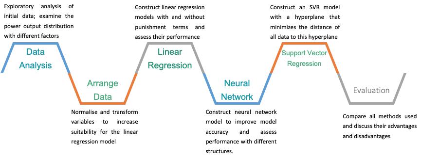
Figure 2: Process for data analysis in this essay.
Model Accuracy Energy Data Analysis代写
Different researchers use different evaluating methodology of their forecasting techniques. Due to the fact that solar output predicting accuracy is dependent on location and time, different error metrics are used across research. In this essay accuracy of the models and comparison among forecasts were estimated by model estimators R2(R-squared) and mean absolute percentage error (MAPE).
R-squared is the traditional statistical metrics for evaluating model quality which can be estimated as following:
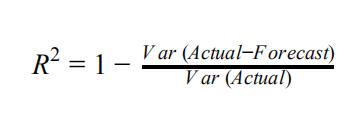
R-squared compares the variances of the error and modelled data and measures the goodness-of-fit for regression analysis. The higher the R2 the lower the more accurate the predictions (Inman et. al. , 2013).Energy Data Analysis代写
MAPE can be expressed as following:
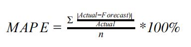
The smaller the value of MAPE the better the forecast. A MAPE score of under 10% is considered highly accurate in forecasting. MAPE is widely used in forecasting as it provides the errors in percentages and avoids issue of positive and negative values cancelling (Kim and Kim, 2016). Assessing the accuracy evaluation metrics plays a crucial role in establishing the most accurate method for forecasting solar output.
The simplest predictive model – Linear Regression (LR) was applied to compute the strength of relationship between variables.
LR estimates the relationship between dependent and independent variables using regression line. Regression has advantages on prediction modelling regarding modelling exogenous variables, which can be formulated with Y as dependent variable as:Energy Data Analysis代写
Y = β0 + β1x1 + β2x2 + … + βnxn
Based on the data analysis, the linear regression model will be tried to built with weather elements to increase the prediction effect. Any new variable will increase the R-squared metric in theory.
Ridge Regression is a example of penalized linear regression,
which regulates overfitting by penalizing the sum of the squared regression coefficients (Bowles, 2015). The linear regression formulation has a low bias, but it is susceptible to high variance or overfit as we increase the number of features. To solve this a penalty term is added in to limit the value of coefficients for lower variance. Meanwhile, ridge regression is a technique used when the data suffers from multicollinearity (independent variables are highly correlated). In multicollinearity, even though the least squares estimates (OLS) are unbiased, their variances are large which deviates the observed value far from the true value. By adding a degree of bias to the regression estimates, ridge regression reduces the standard errors.Energy Data Analysis代写
Instead of lasso regression,
the ridge regression is selected there to get a closed form solution due to the linear operator. Also, there are two methods to choose the coefficient of the penalisation term (lambda): the minimum (min) method and the 1 standard error method. The selection of lambda should provide the least sum of error,s while it is always tested for training group. For the purpose of increasing the model adaptability, the value of lambda is always chosen as the minimum error one plus one standard error to perform well with unseen data. In this project, both the minimum value method and 1 standard error method will be included.Energy Data Analysis代写
Artificial Neural Networks (ANNs) are formed from interconnected nodes in multiple layers, which have the ability to learn complex patterns (Ehsan, Simon and Venkateswaran, 2017). Each so-called ‘perceptron’ node takes a number of inputs and emits an output, taking weightings and activation functions into account. The outputs are fed forward into the next one. By accumulating layers of nodes it is straightforward to build the whole artificial neural network. Mellit (2010) has shown that ANNs perform well when forecasting solar irradiance.
For regression rather than classification,
the decision boundary outputs a continuous value instead of a binary output. The error function relates the output and the training data, and can be evaluated with an error function of our choice, in this case mean squared error. Then, the backwards propagation of errors will calculate gradient in the estimation of weights to update a series of better weights, which are calculated iteratively. In this process, the error is computed based on the output and distributed backwards through the networks layers, and the derivative of the error function will be set as zero to find the best iteration direction. After all points are obtained, the model will find the best weights.
Support Vector Regression (SVR) is a supervised learning technique for working with continuous values.
SVR is non-parametric technique that has advantages on performing the non-linear regression. Kazem et. al.(2016) told that the main advantage of SVR method was that this approach minimized the error through iterative training algorithm and maximized the border between hyperplanes. Unlike the simple regression which tries to minimize the error, support vector regression tries to fit error with certain threshold.Energy Data Analysis代写
SVR uses a kernel function to transform the data, by taking the low dimensional input to higher space and giving possible output. Nageem, R. and R, J. (2017) showed the use of SVR in forecasting solar generation for next hour using the present climate features. The SVR analysis identified that climate changes significantly affect the predicted output. The SVR-based forecasts able to generate highly accurate predictions with only weather forecast and panel characteristics. Figure 3 shows the model structure used for SVR and the other regressions.
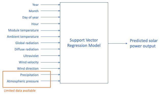
Figure 3. Illustration of model structure
Results
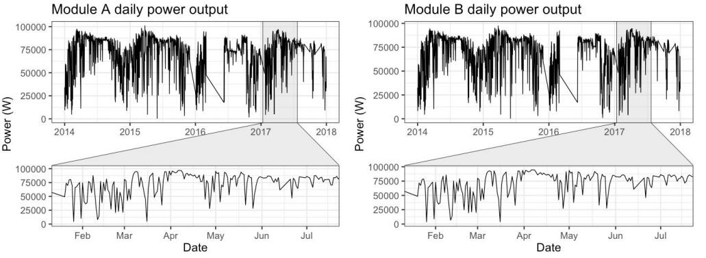
Figure 4: Daily total solar PV power output over four years with detail view
The data features unexplained periods of missing data (see Figure 4);Energy Data Analysis代写
we speculate this could be due to equipment failure, data corruption, or planned interruptions. The missing periods are identical for both module A and B. Environmental data for our other desired environmental factors (module temperature, ambient temperature, global radiation, diffuse radiation, ultraviolet radiation, wind velocity, wind direction) is available over the same time periods with the exception of precipitation and atmospheric pressure.
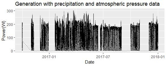
Figure 5: Generation with precipitation and atmospheric pressure, instantaneous readings
EDP did not include precipitation and atmospheric pressure until the end of 2016 (see Figure 5).
Based on the evaluation, the inclusion of precipitation and atmospheric pressure variables clearly increased prediction accuracy. However, the small data size makes the month factor and year day become the principal variables, which leads to a poor prediction and bad model. To solve this problem, the precipitation and atmospheric pressure will not be included, so as to keep the time integrity of data. To ensure maximum effectiveness of our methods all four years of available data is selected. Module angle has a large impact on monthly power output as seen in Figure 6, where horizontally oriented modules show more summertime generation, vertically oriented modules generate more in winter when the sun is lower, and optimally angled panels generate power evenly across the year.Energy Data Analysis代写
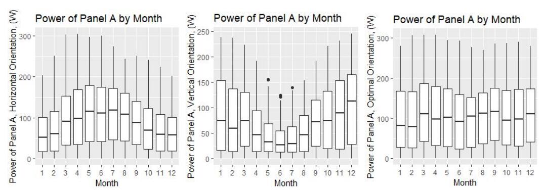
Figure 6: Module A with horizontal, vertical and optimal generation by month
The optimal power generation has been selected for analysis as the evaluation criteria since total generation output is highest: taking the average optimal yearly output as 100%, horizontal and vertical produce 88.3% and 60.8% respectively. Most PV capacity is angled rather than horizontal or vertical which further validates this choice.
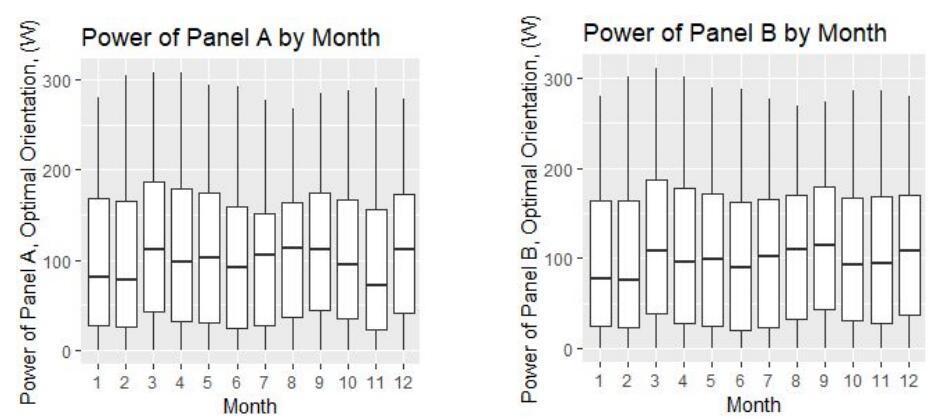
Figure 7: Comparison of Module A and Module B generation by month
Module A and module B show the same trend of generation over time so module A is randomly selected for our analysis. Analysis on the relationship between power generation distribution and each factor is considered.
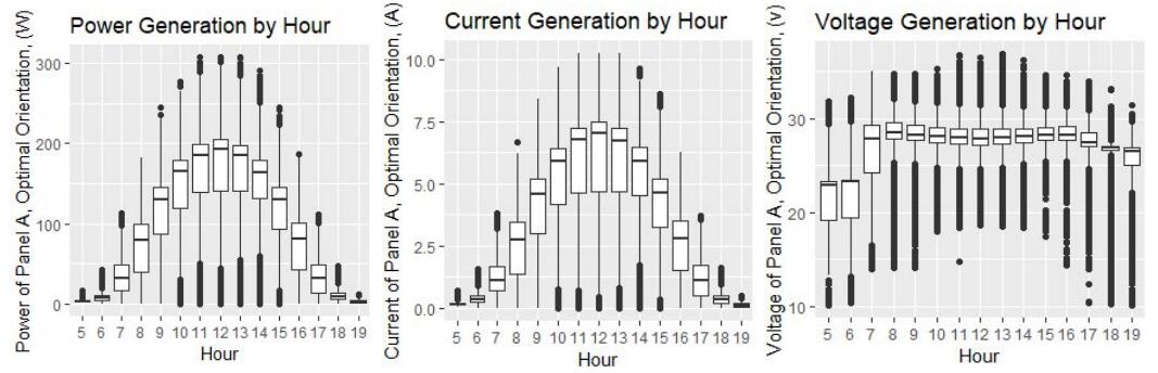
Figure 8: The optional power generation, voltage generation and current generation by hour
The relationship between hour and power generation, current generation and voltage generation are shown in Figure 8. Of course these outputs are tightly related by P = IV. It shows that the voltage generation is relatively stable over the daytime, while current generation and power output are sinusoidal. The reason is straightforwardly that light intensity is correlated closely with the daylight hour.
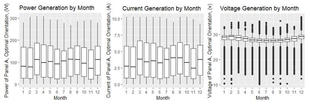
Figure 9: The power generation, voltage and current by month for Panel A in ‘Optimal’ orientation Energy Data Analysis代写
March and September have the largest power generation in this dataset, but the change is not significant across the year (see Figure 9). Meanwhile, the weather data is a key factor.
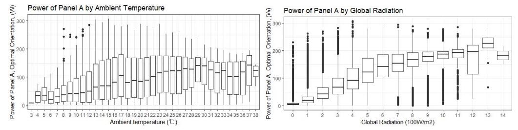
Figure 10: Power generation by ambient temperature and global radiation
The generation keeps increasing with the rising ambient temperature and radiation, while the curve fitting for them are different (see Figure 10). For the ambient temperature, the relationship fairly linear. For global radiation, it flattens after an increasing period which can be fitted as one quarter of a sine function.
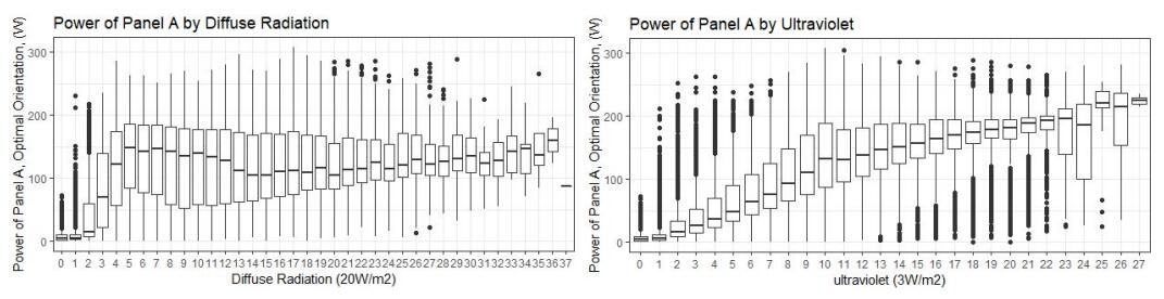
Figure 11: Power generation by diffuse radiation and ultraviolet
The power generation rises with diffuse radiation at the beginning and stays constant as maximum power output is reached. The power generation keeps increasing with ultraviolet as a linear function (see Figure 11).
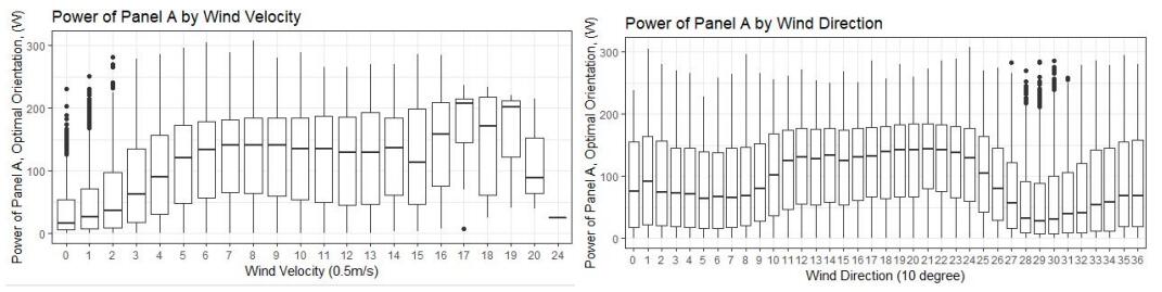
Figure 12: Power generation by wind velocity and direction
The power generation with wind velocity increases at low wind speeds and levels off with a little fluctuation so that this variable seems like a threshold function (see Figure 12). Meanwhile, it actually responds strongly to hourly differences. There is some formulas due to the relationship between wind direction and power generation, this can be done by empirical curve-fitting.Energy Data Analysis代写
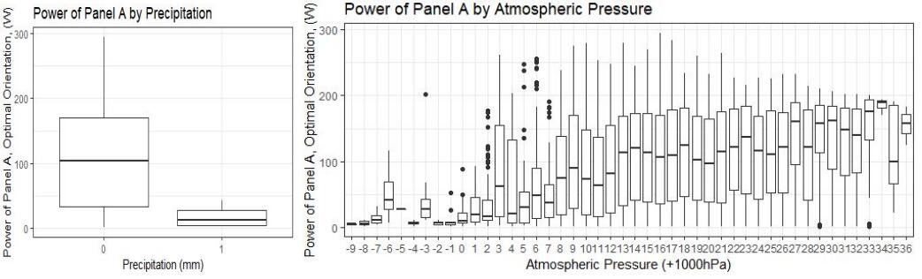
Figure 13: Power generation by precipitation and atmospheric pressure
Precipitation has a strong relationship with power generation (see Figure 13). Increased precipitation strongly reduces power output as might be expected, as rain and clouds obscure any sunlight. The atmospheric pressure increases with a large fluctuation from 1000 hPa to 1034 hPa, with rather unclear behaviour.
Transforming our variablesEnergy Data Analysis代写
Due to the daily and seasonal sinusoidal effects, we transformed many variables including the hour of the day with a fitted function to linearise them against PV power output. The hour variable has no data before 5.00am and after 7.00pm as there was not sufficient generation to be recorded. The transformation addresses the problem with missing hours and removes the discontinuity in the hour variable.
To understand correlation and explore multicollinearity,
the graphs shown in Figure 14 are respectively constructed with original data variables and transformed variables.
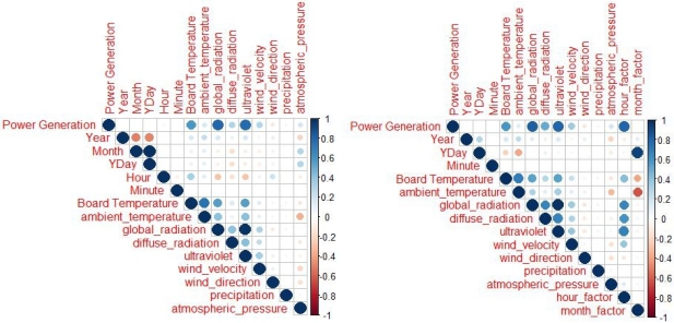
Figure 14: Correlation matrix (left) without function fitting and (right) with transformed independent variables
Based on this analysis, we can decide whether the independent variable need to be transformed. The board temperature, global radiation and ultraviolet are always key factors regardless of transformation. The hour factor and diffuse radiation clearly become more strongly related with the power generation. Meanwhile, some variables are related slightly more with the dependent variable, such as global radiation and ultraviolet. The transform function was created using the MATLAB curve fitting tool. Each function can be given a physical explanation.
Training and test dataEnergy Data Analysis代写
Training error is the error of an estimator as measured by the data used to fit it, which is not a good substitute for prediction error. The test dataset is selected as a separate set of observations to the training data.The training data is selected from 2014 to September 2017, and training data chosen from October 2017 to December 2017. The evaluation will assess average prediction error on the test data as the performance of prediction model.
Linear model results (with and without penalisation term)
The linear regression models provided a range of outputs from quite low accuracies for the simplest linear models to the beginnings of reasonable accuracy with penalised regression. The linear model without penalisation term has been constructed first with training data.
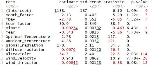
Table 1: Coefficient for each variable in linear regression model without penalisation term
From Table 1,
hour factor, global radiation and ultraviolet are three key factors, whose p-value is very low. Minute is not useful with a 0.643 p-value as it could be during any part of the day. Other variables show little influence on the model, which will fix the prediction in detail.
![]()
Table 2: R squared and adjusted R squared of linear regression model without penalisation term
The adjusted R squared is the same with initial R square as 0.848. The p-value equaling to zero means that the R square is accurate. However, it is just for the training data, so the test data is applied again with predict function and the information is displayed in Table 4.
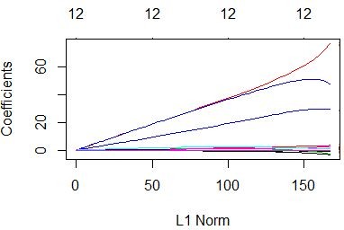
Figure 15: Coefficients function with L1 norm and log Lambda
As the previous model, both the diagrams shows that hour factor, global radiation and ultraviolet really have large influence on linear regression with ridge punishment. The ridge regression will adjust the lambda to the most suitable value as following.Energy Data Analysis代写
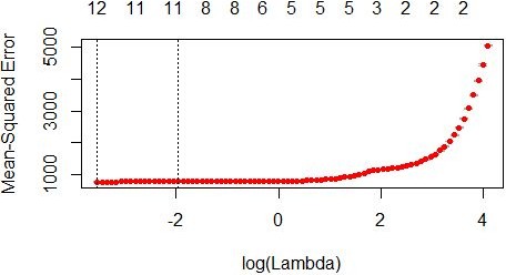
Figure 16: Mean squared error to calculate an optimal lambda term in penalised regression
The lambda for minimum method is 0.029, while it is 0.141 for the one standard error method, which is shown as the red line (see Figure 16). Both the min method and 1 standard error method will used to calculated the prediction value and compared with each other. The one standard error is shown as the grey line, while it is extremely small in this diagram so that the the value of lambda has increased a lot after adding 1 standard error. Based on this point, the result of 1 standard error method is estimated as not very accurate.Energy Data Analysis代写
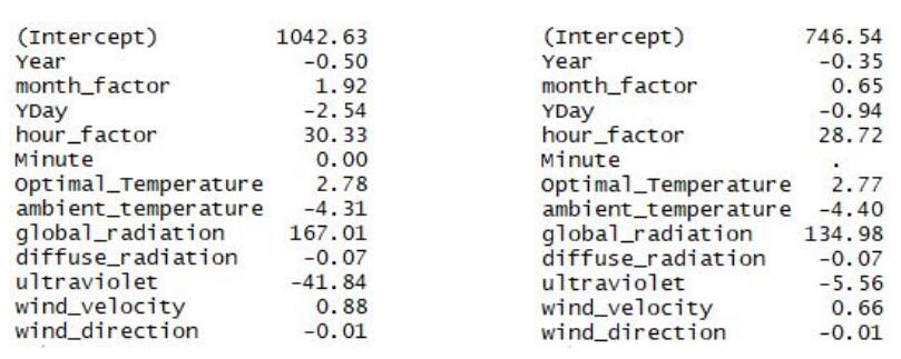
Table 3: Coefficients for each variable in the ridge penalised linear regression for min method (left) and one standard error method (right)
According to the Table 3, the hour factor, global radiation and ultraviolet still have a relatively large coefficient in both two models, which corresponds with the lambda and coefficient graph. They predict the result in test group and the R square and MAPE are shown in Table 4.
ANN Results
As shown in Figure 17, the neural network produces good predictions that respond rapidly to changes in environmental inputs. The model fails to produce consistent low estimates for when the panel is not operating. The data had no values for nighttime periods and filtering to ten minute intervals lost the end of the curve going to zero. Introducing artificial zero values could have addressed this issue.
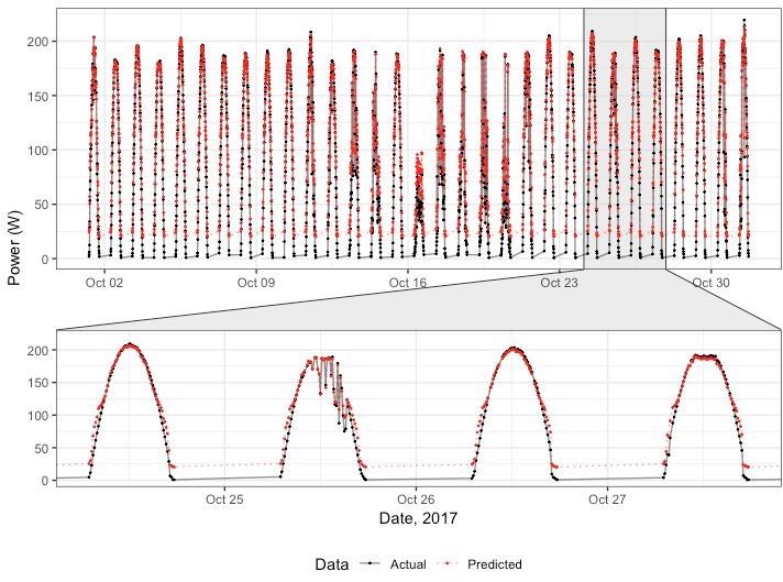
Figure 17: Neural network predictions against actual
SVR Results
Figure 18: Support Vector Regression results plotted against actual generation
The Support Vector Regression (SVR)
performs well with highly variable generation patterns, as shownin Figure 18. The test data are selected as the same as the linear regression method to control conditions.Energy Data Analysis代写
However, the training data size is cut into one tenth filtered by minute to mitigate the huge training time. An SVM regressor was used from the ‘e1071’ R package to apply on the prediction. The R-squared and MAPE are then calculated and shown in Table 4. The test data predictions tends to overestimates the actual generation. As shown before, seasonal output is optimised to produce consistent output but nonetheless as the test data is primarily in the winter of 2017, a seasonal dip could explain the underestimate.
All Results
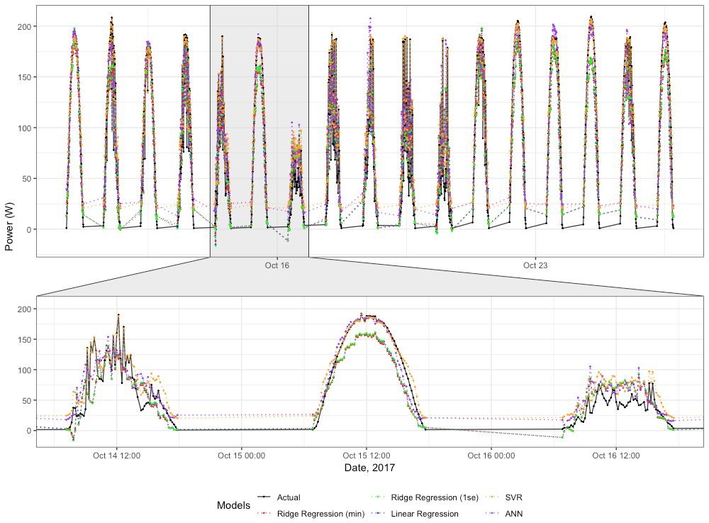
Figure 19: All methods using weather variables inputs plotted over actual generation with detail view
SVR and ANN can be seen to perform well against actual results, while all methods react quickly to changing environmental variables. SVR tends to overestimate output, while the ANN predictions can be very volatile. The linear regression is better than the penalised regression which indicates the coefficients are not large with limited overfitting.Energy Data Analysis代写
| Method | R2 | MAPE | Notes |
| Linear regression (without weather) | 0.563 | 1.92 | Calculated on separate test data |
| Penalised regression (without weather) | 0.555 | 2.05 | Calculated on separate test data |
| Linear regression | 0.839 | 0.587 | Calculated on separate test data |
| Ridge Penalised regression (min method) | 0.836 | 0.593 | Calculated on separate test data |
| Ridge Penalised regression (1se method) | 0.823 | 0.580 | Calculated on separate test data |
| Neural Network (with keras package) | 0.889 | 0.788 | Calculated on separate test data |
| Support Vector Regression | 0.894 | 0.700 | Calculated on separate test data |
Table 4: Results of different methods comparing R-squared and MAPE error metrics
The SVR method obtained the highest R-squared value followed by NN, while the ridge regression (1se method) model achieved the lowest MAPE value, although there was little difference in MAPE score between the simple linear regression model and either penalised regression.Energy Data Analysis代写
The data has no actual generation zero results which would cause the MAPE calculation to fail as those results serve as denominator in part of the calculation, although weighted absolute percentage error (WAPE) could be substituted. MAPE is also known to be biased towards underestimates (Makridakis, S., 1993). Maximising R-squared is equivalent to minimising the mean squared errors (MSE), and considering the above appears the more robust metric here.
Discussion and conclusions
While several approaches yielded accurate results, we found using penalised regression and SVR to be the most accurate methods, depending on error metric, for predicting the SunLab optimally angled PV module generation output for a given time using environmental data. The high correlation between environmental factors like solar irradiation, precipitation, module temperature and the power output of a PV module is of course obvious and unsurprising. What may be of interest is the relatively good accuracy that can be obtained with simple methods based on timely and accurate weather data.
CaveatsEnergy Data Analysis代写
As ever, we can confidently state that more data is required. While the temporal resolution of the data used was comparatively good, significant missing time-periods and a short time range means we can only have limited confidence in the conclusions about modelling approaches to transfer to other PV installations. Simultaneous analysis on a training and test dataset composed of many modules with varying angles, orientations and locations experiencing varied environmental conditions would enhance the strength of conclusions that could be drawn significantly.
More methodological care could have been taken to select error metrics,
for example Inman et al, (2013) notes the use of root mean squared error (RMSE), mean bias error (MBE) and Kolmogorov-Smirnov Integral (KSI) for irradiance model accuracy. While data was filtered to every ten minute value, a more sophisticated aggregation method or leaving the data at one minute values could have yielded better results at the cost of computation time which could have been addressed with better planning or more resources. More care could have been taken to use adjusted R-squared metrics. While multiple recent studies suggested hybrid approaches for forecasting techniques, this was not something we were able to implement in this essay.Energy Data Analysis代写
Generalisability
The generalisability of these methods depends on the availability of quality forecasts of weather data. Commercial and publicly available weather forecasts usually contain pressure data, precipitation, UV, ambient temperature and wind, which along with the time of day factor supplied most of the accuracy in our predictions. What is significantly challenging is the temporal resolution of these forecasts. In particularly, partly cloudy days can result in very variable PV module output as direct irradiance changes rapidly.
As mentioned in introduction achieving highly accurate prediction of solar PV output is crucial for development of solar power generation.
Over a yearly basis this is clearly possible to a good accuracy and therefore from a PV project developer’s perspective calculating potential output is straightforward. From a power systems planning or grid operator perspective, the varying generation output from solar PV continues to be challenging (Lin and Pai, 2016). However, weather forecasts become more accurate the smaller the time horizon and high accuracy forecasts can be expected for time periods up to one day away, which may address this issue and enable accurate PV generation forecasts to be calculated.Energy Data Analysis代写
Future work
Future work could include more datasets and assess differences and similarities across module technologies, optimal angles and orientations for modules in different geographical locations, module ages and degradation. A comparison of the availability and accuracy of weather forecast data would be a worthwhile exercise given the importance it has to accurate PV generation forecasts that we have outlined. More analysis of seasonality and autocorrelation of time-series data could prove fruitful as a different approach. Other models like LSTMs, more sophisticated neural networks and hybrid approaches could yield better results, although the number of independent variables in our prediction model in this essay could mean high computational costs. Remote monitoring could be an interesting tool as mentioned previously as satellite imagery data becomes increasingly available.
References Energy Data Analysis代写
Abuella, M., & Chowdhury, B. (2015). Solar power probabilistic forecasting by using multiple linear regression analysis. SoutheastCon 2015, 2015(June), 1-5.
Antonanzas, J., Osorio, N., Escobar, R., Urraca, R., Martinez-de-Pison, F. and Antonanzas-Torres, F. (2016). Review of photovoltaic power forecasting. Solar Energy, 136, pp.78-111.
Bouzerdoum, M., Mellit, A., Pavan, A.M., 2013. A hybrid model (SARIMA–SVM) for short-term power forecasting of a small-scale grid-connected photovoltaic plant. Solar Energy 98, 226–235.Energy Data Analysis代写
Bowles, M. (2015). Machine learning in python : Essential techniques for predictive analysis.
Deo, R. and Şahin, M. (2017). Forecasting long-term global solar radiation with an ANN algorithm coupled with satellite-derived (MODIS) land surface temperature (LST) for regional locations in Queensland. Renewable and Sustainable Energy Reviews, 72, pp.828-848.
EDP, 2019. Sunlab — EDPOpenData [online]. Available at https://opendata.edp.com/pages/sunlab/ (accessed 1.13.19).
Hammer, Heinemann, Lorenz, & Lückehe. (1999). Short-term forecasting of solar radiation: A statistical approach using satellite data. Solar Energy, 67(1), 139-150.
Huang, R., Huang, T., Gadh, R., Li, N., 2012. Solar generation prediction using the ARMA model in a laboratory-level micro-grid, in: Smart Grid Communications (SmartGridComm), 2012 IEEE Third International Conference On. IEEE, pp.
528–533.
Inman, R. H., Pedro, H. T., & Coimbra, C. F. (2013). Solar forecasting methods for renewable energy integration. Progress in Energy and Combustion Science, 39(6), 535-576.Energy Data Analysis代写
Ji, W. and Chee, K. (2011). Prediction of hourly solar radiation using a novel hybrid model of ARMA and TDNN. Solar Energy, 85(5), pp.808-817.
Kazem, Hussein A & Yousif, Jabar & Chaichan, Miqdam. (2016). Modelling of Daily Solar Energy System Prediction using Support Vector Machine for Oman.
International Journal of Applied Engineering Research. 11. 10166-10172.
Kim, S. and Kim, H. (2016). A new metric of absolute percentage error for intermittent demand forecasts. International Journal of Forecasting, 32(3), pp.669-679.
King, D.L., Boyson, W.E., Kratochvil, J.A., 2002. Analysis of factors influencing the annual energy production of photovoltaic systems, in: Photovoltaic Specialists Conference, 2002. Conference Record of the Twenty-Ninth IEEE. IEEE, pp. 1356–1361.
Lin, K. and Pai, P. (2016). Solar power output forecasting using evolutionary seasonal decomposition least-square support vector regression. Journal of Cleaner Production, 134, pp.456-462.Energy Data Analysis代写
Liu, B. and Jordan, R. (1960). The interrelationship and characteristic distribution of direct, diffuse and total solar radiation. Solar Energy, 4(3), pp.1-19.
Makridakis, S., 1993. Accuracy measures: theoretical and practical concerns.
International Journal of Forecasting 9, 527–529.
Mandal, P., Madhira, S., haque, A., Meng, J. and Pineda, R. (2012). Forecasting Power Output of Solar Photovoltaic System Using Wavelet Transform and Artificial Intelligence Techniques. Procedia Computer Science, 12, pp.332-337.
Marvin, C. and Kimball, H. (1926). Solar radiation and weather forecasting. Journal of the Franklin Institute, 202(3), pp.273-306.
Mathiesen, P., Collier, C., Kleissl, J., 2013. A high-resolution, cloud-assimilating numerical weather prediction model for solar irradiance forecasting. Solar Energy 92, 47–61.Energy Data Analysis代写
Mellit, A. (2010). A 24-h forecast of solar irradiance using artificial neural network: Application for performance prediction of a grid-connected PV plant at Trieste, Italy. Solar Energy, 84(5), 807-821.
Muhammad Ehsan, R., Simon, S., Venkateswaran, P. (2017). Day-ahead forecasting of solar photovoltaic output power using multilayer perceptron. Neural Computing and Applications, 28(12), 3981-3992.
Mutoh, N., Matuo, T., Okada, K., Sakai, M., 2002. Prediction-data-based maximum-power-point-tracking method for photovoltaic power generation
systems, in: Power Electronics Specialists Conference, 2002. Pesc 02. 2002 IEEE 33rd Annual. IEEE, pp. 1489–1494.
Nageem, R. and R, J. (2017). Predicting the Power Output of a Grid-Connected Solar Panel Using Multi-Input Support Vector Regression. Procedia Computer Science, 115, pp.723-730.
Qazi, A., Fayaz, H., Wadi, A., Raj, R., Rahim, N. and Khan, W. (2015). The artificial neural network for solar radiation prediction and designing solar systems: a systematic literature review. Journal of Cleaner Production, 104, pp.1-12.
Shang, C. and Wei, P. (2018). Enhanced support vector regression based forecast engine to predict solar power output. Renewable Energy, 127, pp.269-283.
Sobri, S., Koohi-Kamali, S. and Rahim, N. (2018). Solar photovoltaic generation forecasting methods: A review. Energy Conversion and Management, 156, pp.459-497.Energy Data Analysis代写
Spencer, J. (1982). A comparison of methods for estimating hourly diffuse solar radiation from global solar radiation. Solar Energy, 29(1), pp.19-32.
Wang, G., Su, Y. and Shu, L. (2016). One-day-ahead daily power forecasting of photovoltaic systems based on partial functional linear regression models. Renewable Energy, 96, pp.469-478.
Yang, D., Kleissl, J., Gueymard, C., Pedro, H. and Coimbra, C. (2018). History and trends in solar irradiance and PV power forecasting: A preliminary assessment and review using text mining. Solar Energy, 168, pp.60-101.
Supplementary material
Datasheet for PV Module A: https://github.com/Rabscuttler/solar_PV_forecasting/blob/master/datasheets/ModuleA_Datasheet.pdf
Datasheet for PV Module B: https://github.com/Rabscuttler/solar_PV_forecasting/blob/master/datasheets/ModuleB_Datasheet.pdf Energy Data Analysis代写
Atmospheric pressure, ambient temperature, wind speed, wind direction and precipitation taken by Vaisala Weather Transmitter WXT520: https://www.vaisala.com/sites/default/files/documents/M210906EN-C.pdf
Solar measurements taken using a DELTA-T Sunshine Pyranometer SPN1: https://www.delta-t.co.uk/wp-content/uploads/dlm_uploads/2017/05/SPN1-UM-4.1.pdf
UV measurements taken using a Kipp & Zonen CUV5 UV Radiometer: http://www.kippzonen.com/Product/163/CUV5-UV-Radiometer#.WuyU-Grwb4Y

更多其他:C++代写 考试助攻 计算机代写 report代写 project代写 数学代写 java代写 程序代写 algorithm代写 r代写 北美代写 代写CS 代码代写 金融经济统计代写 function代写
