
MSc ESDA Coursework Title Page
Energy Analytics代写 By submitting this document, you are agreeing to the Statement of Authorship:I/We certify that the attached coursework
The Bartlett School of Environment, Energy and Resources
UCL Candidate Code: Module Code: Module Title: Coursework Title: Module Leader: Date:
Word Count:
CHTL0 BENV0092
Energy Analytics in the Built Environment
Cluster Analysis for the Characterisation of Heat Pump Demand Profiles
Despina Manouseli 09/01/2019
Word Count :2,932
By submitting this document, you are agreeing to the Statement of Authorship:
I/We certify that the attached coursework exercise has been completed by me/us and that each and every quotation, diagram or other piece of exposition which is copied from or based upon the work of other has its source clearly acknowledged in the text at the place where it appears.Energy Analytics代写
I/We certify that all field work and/or laboratory work has been carried out by me/us with no more assistance from the members of the department than has been specified.
I/We certify that all additional assistance which I/we have received is indicated and referenced in the report.
Please note that penalties will be applied to coursework which is submitted late or which exceeds the maximum word count. Information about penalties can be found in the MSc ESDA Course Handbook which is
available on Moodle:
- Penalties for late submission:https://moodle-1819.ucl.ac.uk/course/view.php?id=9967§ion=30
- Penalties for going over the word count:https://moodle-1819.ucl.ac.uk/course/view.php?id=9967§ion=30
In the case of coursework that is submitted late and is also over length, then the greater of the two penalties shall apply. This includes research projects, dissertations and final reports.Energy Analytics代写
Cluster Analysis for the Characterisation of Heat Pump Demand from a UK Field Trial
Introduction Energy Analytics代写
Heat accounts for nearly half of final energy consumption in the UK (44% or 59,000 tonnes of oil equivalent) with two thirds of this demand being met by gas (BEIS, 2018a). The decarbonisation of heat therefore will be central to meeting the UK’s ambition of an 80% reduction of greenhouse gas emission by 2050.
Heat pumps are one of the key technologies that the UK Government
is supportive of to decarbonise the provision of heat and hot water in UK homes and businesses. Uptake of heat pumps along with other renewable heat technologies has been encouraged through the Renewable Heat Incentive (RHI). The scheme was first implemented in 2014 and so far has supported the installation of around 28,000 domestic and 1,500 non-domestic heat- pumps (BEIS, 2018b). In 2016 the government revised the scheme, increasing the tariff rates to further stimulate uptake (BEIS, 2016). Successful uptake coupled with decarbonisation of electricity has the potential to significantly reduce carbon emissions from heat (Luickx,
Helsen and D’haeseleer, 2008). Initial focus has been areas that are off the gas grid, representing 18% of households in 2050 (Strbac et al., 2018). However, addressing heat demand in the remaining households will also be necessary to meet emissions targets. A recent scenario analysis for decarbonising heat found that both electric pathways which make greater use of heat pumps, and hybrid scenarios use Hydrogen and carbon-neutral gas, have the greatest potential to
reduce emissions to zero at a reasonable cost (Strbac et al., 2018) (Figure 1). Energy Analytics代写
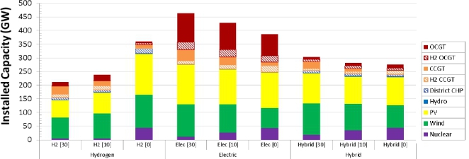
Figure 1: Optimal generation portfolio for core decarbonisation pathways from (Strbac et al., 2018). 30, 10 and 0 are different carbon targets the number being Mt of carbon
However,
there are significant barriers to largescale uptake of heat pumps and realising emissions reductions. From a household perspective these include the high up-front cost, high relative cost of electricity versus gas and high home energy efficiency required for effective operation (Committee on Climate Change, 2018). From a system perspective the challenges are also considerable. The large seasonal demand means that transferring from fuels to electricity adds considerably to the requirements from the grid. Love et al., (2017) estimate that peak grid demand increases by 7.5 GW (14%) when penetration of heat pumps in households reaches 20%.
Load profiles for heat pumps do not match that for heat from fuels or other electricity demand (Love et al., 2017). Having a better understanding of the variation in theses profiles helps to construct a more detailed picture of aggregate demand, better focussing technological and policy developments needed to meet the specifics of these demands.
This paper focusses on developing a more granular understanding of demand for electricity of heat pump systems through an analysis of load data from field trial data for heat pumps installed under the RHI between 2011 and 2015.
Literature Review Energy Analytics代写
Empirical data for electricity demand from heat pumps has not been frequently collected and therefore previous studies have largely used modelled data for electricity usage based on heat demand. This approach requires that heat loads are estimated adding further uncertainty. Demand may be estimated from current loads where they are known or through further simulation such as by developing a building physics model (Harkin and Turton, 2017) or by creating a simplified heat load profile (Luickx, Helsen and D’haeseleer, 2008).
The operation of heat pumps to meet this demand must then be simulated and resulting load estimated. Energy Analytics代写
Navarro-Espinosa and Mancarella (2014) take a probabilistic approach using Monte Carlo simulation to create ‘black-box’ models representing ground and air source heat pumps (GSHP and ASHP) that transform heat demand into power demand. The aggregation of a diverse set of simulated profiles has also been used in a number of studies to estimate system wide demands from heat pumps (Navarro-Espinosa and Mancarella, 2014).
When directly measured consumption data is available, other techniques become possible. For example a study from Beijing, China uses data mining and machine learning techniques to forecast month ahead demand for a water source heat pump based on 5-minute interval consumption and weather data (Ahmad, Chen and Shair, 2018). Clustering is a frequently used method to analyse load profiles as it allows complex data with high dimensionality to be grouped into clusters that have common characteristics, for example (Bobric, Cartina and Grigoraş, 2009; Deepak Sharma and Singh, 2014).Energy Analytics代写
Because of the limited availability of granular load data,
cluster analysis specific to heat pumps is less common. Two relevant examples were found in the literature. Firstly in Wallnerström et al. (2014) seek to identify when residential customers in Finland switch from conventional heating system to GSHP and produce grouping of these customer through clustering of hourly load data. In it they use K-means and principal component
analysis, but wasn’t successful in distinguishing GSHP compared electric heating customers. This may be in part due to the granularity of the data. In Do Carmo and Christensen (2016) heat load data is analysed using from hourly data from 139 dwellings in Denmark with the aim of creating a typology of load profiles. K-means clustering is used to firstly group into period of low, medium and high demand for each household then to characterise load within these segments. The difference in clusters are found to be related to particular building characteristics like house area, building age and radiator type.Energy Analytics代写
Methodology
This study makes use of field trial data for around 400 ASHPs and GSHPs that includes 2- minute interval data for temperature and power use (Summerfield et al., 2016). This data was chosen as it is unique in the sample size and granularity of measurements. Studies based on the data set so far have focussed on performance of the heat pump systems (Summerfield et al., 2016) and calculating After Diversity Maximum Demand (ADMD).
Instead of taking a generative approach to analysing demand,Energy Analytics代写
this study makes use of unsupervised machine learning techniques (clustering) to characterise different demand profiles. To create insight into these profiles, explanatory models will be tested using supervised approaches. All using R programming language.
There are a wide range of clustering techniques available including k-means, hierarchical, Gaussian mixture models, spectral and linear discriminant analysis. Two different methods are tested, comprising of k-means and spectral clustering. K-means is a commonly used algorithm where the user specifies the number of clusters and the algorithm iterates between (1) assigning each data point to a cluster based on Euclidean distance, and (2) recalculating cluster centroids based on these allocations until the distances for each data point to its cluster centroid (distortion) is minimised as much as possible. Because the centroids are randomly initialised, the algorithm can produce different results depending on the starting position. Picking the optimal number of clusters is done by validating the distortion factor against cluster number.Energy Analytics代写
Spectral clustering uses spectral graph partitioning, taking on three main steps. Firstly, creating a matrix representation of the graph, secondly perform an Eigen decomposition of this affinity matrix mapping each point to its lower dimension representation, and finally assign groups to clusters based on the new representation. This last step makes use of the coordinates of Eigen decomposition and uses k-means to create the clustering (Von Luxburg, 2007).
One of the challenges with clustering or unsupervised techniques is analysing performance
i.e. how well has the chosen technique and application described the data. To overcome this, an explanatory modelling (regression) was used based on other metadata and summary consumption data for each household. This allows the interpretation of the clusters in relation to other characteristics of the dwelling or consumption profile. Because the clustering results in discrete nominal variables multinomial logistic regression is used with the cluster grouping as the independent variable. An example of this approach is found in Andresen (2015) where they use population statistics to predict crime clusters in Vancouver, British Columbia.
The original data from the trial produced readings for 699 sites. In this analysis a cleaned dataset created for the initial analysis is used that consists of 418 sites. Sites excluded from this dataset due to technical issues relating to the installation of water temperature sensors or because of missing data streams. See (Summerfield et al., 2016) for more details.Energy Analytics代写
As in (Love et al., 2017) this analysis focuses on the ‘Ehp’ measurements, which are those taken for electricity use of the heat pump unit alone rather than wider system use e.g. for immersion heaters or system boost.
This corresponds to the H2 system boundary elaborated in the schematic below.
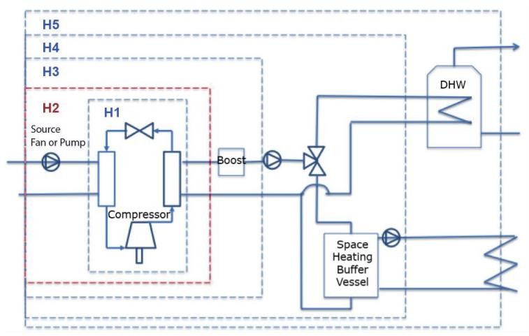
Figure 2: Idealised schematic for a heat pump showing the H1-H5 boundaries. Taken from Lowe et al., (2017)
In order to have comparable data when all heat pumps had readings, a limited time period was selected for the cluster analysis. The month of May 2014 was chosen and just weekdays selected for simplicity. Even limited to this period this still created upwards of 22,000 readings per site. Having removed sites where not enough data was available in the period left 306 sites for analysis. For the purpose of clustering any remaining missing values were estimated using linear interpolation. On completion of the cluster analysis the cluster groupings were added to the site metadata and summary performance measures created by Lowe et al. (2017).
Analysis and Results
Cluster analysis
K-means
Having run the k-means algorithm the following plot of distortion (total within sum of squares) was derived for different cluster numbers (k) (Figure 2). The optimal value of K is normally taken as the point where increasing the number of clusters doesn’t provide significantly more value in reducing the distortion. However, in Figure 2 the slope is fairly continuous. Based on the small break after k=5, k was chosen to be 6.
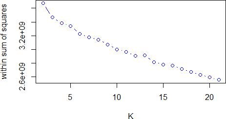
Figure 2: Plot of distortion against number of clusters (K) for k-means for weekdays in May 2014
The six clusters were assigned to each site record and mean consumption at 2 minute intervals for all data was calculated. Figure 3 below shows the average profile for each cluster. From visual inspection the difference between the clusters mostly relates to the magnitude of consumption with some clusters showing some variation in peak consumption. Cluster 3 in particular has a morning peak that is earlier than for the other clusters whilst the peaks for clusters 4 and 6 are much less distinct.
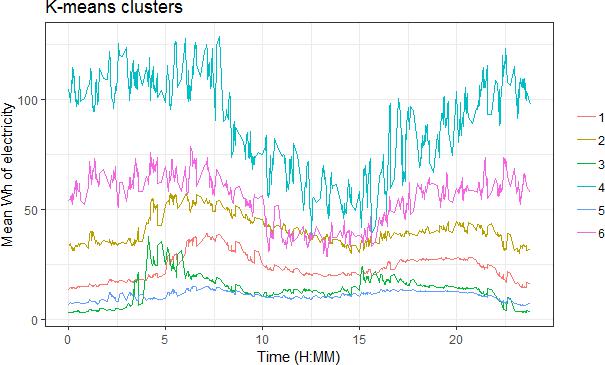
Figure 3: Mean Wh of electricity usage at 2-minute intervals for weekdays in May 2014 for heat pump clusters derived using k-means.
Spectral clustering
The spectral cluster algorithm was run on the same data. The algorithm indicates the optimal number of clusters by choosing the Eigen value based on the Eigen gap heuristic (Von Luxburg, 2007). This is based on the idea that it is optimal to choose a value of k such that the Eigen values �1 … … �� are small, but ��+1 is relatively large. The red line in Figure 4 below shows that this analysis using the Eigen gap heuristics gives and optimal number of clusters of 2.
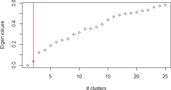
Figure 4: Plot of Eigen values against number of clusters from specClust the spectral clustering algorithm
When plotted for mean consumption this gives two very similar profiles where the main difference is the magnitude of consumption. Whilst this is an interesting finding in itself it does not provide much insight into possible differences in consumption.
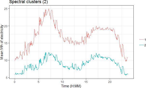
Figure 5: Mean Wh of electricity usage at 2-minute intervals for weekdays in May 2014 for heat pump clusters derived using spectral clustering (optimum choice).
Based on Figure 4 there are no other major breaks of slope of the Eigen values, so in order to further evaluate what natural clusters might exist the between cluster distances were plotted against k. On examination of this there is considerable increase in the sum of squared distances between clusters for k<6 after which there is much less improvement.
Based on this 6 clusters were plotted (see Figure 6). On visual inspection the cluster profiles show more variability between clusters, but also temporal variance within clusters is greater than for k-means. The timing of peak demand is quite different between the clusters.Energy Analytics代写
Analysis of counts of sites in each cluster (Table 1) shows that with six clusters, some clusters have a small number of sites. This is particularly true of k-means where clusters 4 and 6 have just one site each. The spectral 6 clustering represents an improvement on this having a minimum of seven sites in a cluster. A spectral clustering with four clusters was also run for comparison. Interestingly this is less balanced than that with six clusters.
| Cluster number | k-means | Spectral 6 clusters | Spectral 4 clusters | Spectral 2 clusters |
| 1 | 63 | 94 | 103 | 231 |
| 2 | 8 | 7 | 4 | 75 |
| 3 | 37 | 30 | 196 | |
| 4 | 1 | 100 | 3 | |
| 5 | 196 | 63 | ||
| 6 | 1 | 12 | ||
| Total | 306 | 306 | 306 |
Table 1: Count of heat pump sites in each cluster for k-means and spectral clustering.
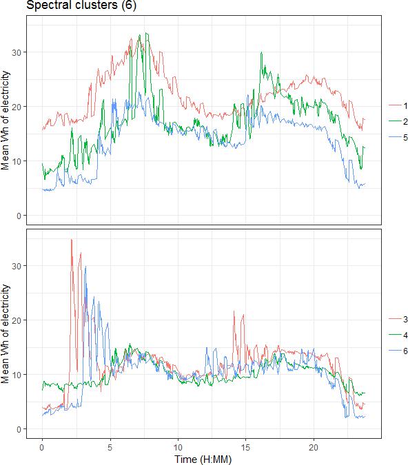
Figure 6: Mean Wh of electricity usage at 2-minute intervals for weekdays in May 2014 for heat pump clusters derived using spectral clustering (k=6).
Regression analysis Energy Analytics代写
To improve the interpretability of the clusters and to further assess their validity, clusters were combined with metadata for each site and with summary consumption data and seasonal performance estimates for the whole trial period. The aim of the analysis is to see if regression analysis can be used to predict each sites membership of the derived clusters based on these characteristics. Exploratory heat plots show some potentially interesting patterns that were tested through later regression (Figure 7).
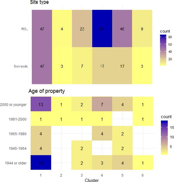
Figure 7: Example heat maps of cluster groupings with metadata (spectral 6)
In order to perform regression where the cluster is the dependent variable, a multinomial logistic regression function was used as this allows prediction of categorical variables.Energy Analytics代写
Because of the low number of sites in some of the k-means clusters the k-means clusters weren’t used. After checking for correlation amongst the independent variables a number of models were run using the mlogit algorithm and the outputs were assessed on two levels.
Firstly the performance of the whole model was interpreted using the pseudo R-squared value (McFadden test), the likelihood ratio test (chi-squared) and associated p-values.
Secondly, for better fitting model the independent variables were assessed. An example output of the model is included below for reference (Figure 2).
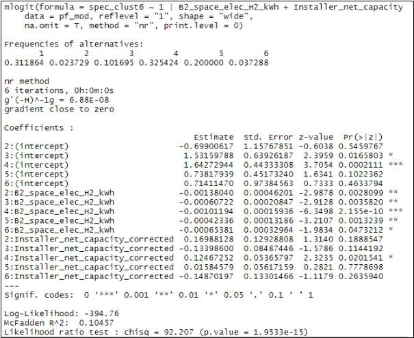
Figure 8: Model summary produced by the mlogit function
A selection of the models run are included in Table 2 below. Of these models those that included both summary consumption measures (e.g. seasonal performance factor, electricity consumption for space and water), pump setup and dwelling characteristics had the greatest explanatory power with the best performing. Those with just pump setup or just dwelling characteristics did not perform as well. The best performing models achieved a pseudo R-squared value of around 0.2.
| # | Model formula Energy Analytics代写 | Log- Likelihood | McFadden R^2 | Chi-squared
– likelihood ratio test |
p-value |
| 1 | spec_clust6 ~ 1 | B2_space_elec_H2_kWh + B2_SPF_H2
+ B2_Water_elec_H2_kWh + Installer_net_capacity_corrected |
-362.65 | 0.17531 | 154.19 | 2.22E-16 |
| 2 | spec_clust6 ~ 1 | B2_space_elec_H2_kWh + B2_SPF_H2
+ B2_Water_elec_H2_kWh |
-390.03 | 0.14506 | 132.36 | 2.22E-16 |
| 3 | spec_clust6 ~ 1 | Emitter_type + Heat_pump_type +
Site_type + Schematic_as_documented |
-431.59 | 0.056302 | 51.498 | 0.001387 |
| 4 | spec_clust6 ~ 1 |
B2_space_elec_H2_kWh |
-394.76 | 0.10457 | 92.207 | 1.95E-15 |
| 5 | spec_clust6 ~ 1 | B2_space_elec_H2_kWh + B2_SPF_H2
+ B2_Water_elec_H2_kWh + Installer_net_capacity_corrected + Installer_annual_generation_corrected |
-352.38 | 0.19653 | 172.39 | 2.22E-16 |
| 6 | B2_space_elec_H2_kWh + B2_SPF_H2
+ B2_Water_elec_H2_kWh + Installer_net_capacity_corrected + Installer_annual_generation_corrected + Heat_pump_type + Site_type + Schematic_as_documented Energy Analytics代写 |
-344.57 | 0.21434 | 188.01 | 2.22E-16 |
Table 2: Model performance parameters for a selection of models using mlogit
Looking in more detail at the best performing of the models (number 6) we can further interpret the effect of each independent variable on predicting each of the clusters. For example, electricity used for space heating all had negative coefficients when the reference case was cluster 1 (all with p-values much smaller than 0.05), meaning that as usage goes up the likelihood of the site being any cluster goes down compared to cluster 1 (reference case). Conversely the when cluster 4 is the reference case increasing usage increases the likelihood that it is in clusters 1 and 5 (p-values < 0.05). This feature is reflected in Figure 9 below.
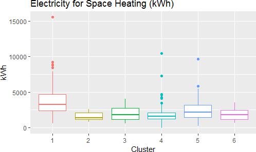
Figure 9: Plot of modelled electricity use for space heating for each cluster (spectral 6)Energy Analytics代写
By comparison, for water heating the most significant differences are seen in the coefficients when the reference case is set to cluster 2 with all but cluster 1 having negative coefficients (p-value <0.05). This can also be seen graphically in Figure 10.
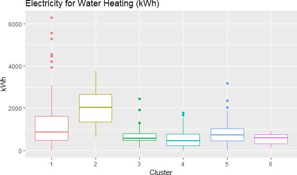
Figure 10: Plot of modelled electricity use for space heating for each cluster (spectral 6)
Discussion and Conclusion Energy Analytics代写
The aim of this analysis was to investigate if there are diverse groups of load profiles of heat pumps in the UK and does the related metadata predict what these groups are.
The clustering techniques (k-means and spectral)
produced some distinct clusters of demand profile that do have some diversity in magnitude and timing. On closer inspection the results of the k-means clustering were not useable as it resulted in some clusters with just one member. The spectral clustering produced improved results, however further analysis is needed to understand them better. For example, looking at within cluster variance for aggregated time periods might clarify the extent to which clusters are homogenous.
Creating a predictive model for the spectral 6 clusters was successful in achieving a pseudo R-squared score of greater than 0.2. Combinations of independent variables for dwelling characteristics, pump setup and consumption in combination created the strongest models. Looking in more depth at the independent variables and their relationship with each cluster, electricity consumption for water and space heating were found to be strong predictors of cluster 2 and 1 respectively. In this sense the analysis may be considered sufficiently successful.Energy Analytics代写
However,
for this type of analysisto be of greater use, stronger prediction of clusters based on characteristics more extraneous to the heating system would be preferable. Plotting of the metadata against the spectral 6 clusters appeared to show some difference between clusters (Figure 7), but this was not supported by the regression. One limitation is that the metadata is incomplete compared to the raw consumption data, which places a limitation on the regression analysis.
It should be noted that the sample of heat pump sites is not representative of the wider building stock – two thirds of the sites were registered social landlords compared to around one sixth of all households (HCLG, 2018). A further representation limitation of using this sample is that it only includes installations where they replace older heating systems.Energy Analytics代写
There were also limitations to the analysis carried out on the dataset due to heavy processing requirements associated with the high granularity. The performance of cluster analyses for weekdays, weekends and for other periods not covered in this study would be beneficial for creating a more complete picture. The creation of more latent variables from the consumption data such as variance, max, min standard deviation for different time brackets may improve the modelling in the second part of this analysis.
Overall the approach used here has identified a number of merits, and future work may seek to refine the process, by exploring different clustering techniques, creating latent variables or by applying the same techniques to more comprehensive data.
References Energy Analytics代写
Ahmad, T., Chen, H. and Shair, J. (2018) ‘Water source heat pump energy demand prognosticate using disparate data-mining based approaches’, Energy. Elsevier Ltd, 152, pp. 788–803. doi: 10.1016/j.energy.2018.03.169.
Andresen, M. A. (2015) ‘Predicting Local Crime Clusters Using ( Multinomial ) Logistic Regression’, Cityscape: A Journal of Policy Development and Research, 17(3), pp. 249–262.
BEIS (2016) ‘The Renewable Heat Incentive: A Reformed Schreme’, (December). Available at: https://www.gov.uk/government/uploads/system/uploads/attachment_data/file/577024/R HI_Reform_Government_response_FINAL.pdf.
BEIS (2018a) Energy Consumption in the UK. Available at: https://www.gov.uk/government/statistics/energy-consumption-in-the-uk (Accessed: 2January 2019).Energy Analytics代写
BEIS (2018b) RHI monthly official statistics tables Nov 2018. Available at: https://www.gov.uk/government/statistics/rhi-monthly-deployment-data-november-2018 (Accessed: 29 December 2018).
Bobric, E. C., Cartina, G. and Grigoraş, G. (2009) ‘Clustering techniques in load profile analysis for distribution stations’, Advances in Electrical and Computer Engineering, 9(1), pp. 63–66. doi: 10.4316/aece.2009.01011.
Do Carmo, C. M. R. and Christensen, T. H. (2016) ‘Cluster analysis of residential heat load profiles and the role of technical and household characteristics’, Energy and Buildings.Energy Analytics代写
Elsevier B.V., 125, pp. 171–180. doi: 10.1016/j.enbuild.2016.04.079.
Committee on Climate Change (2018) ‘Reducing UK emissions – 2018 Progress Report to Parliament -’, Committee on Climate Change, (June). doi: 10.1111/j.1530- 0277.1986.tb05619.x.
Deepak Sharma, D. and Singh, S. N. (2014) ‘Electrical load profile analysis and peak load assessment using clustering technique’, IEEE Power and Energy Society General Meeting. IEEE, 2014–Octob(October), pp. 1–5. doi: 10.1109/PESGM.2014.6938869.
Harkin, S. and Turton, A. (2017) ‘Managing the future network impact of the electrification of heat’, CIRED – Open Access Proceedings Journal, 2017(1), pp. 1888–1891. doi: 10.1049/oap-cired.2017.1123.
HCLG (2018) ‘English Housing Survey – Social rented sector, 2016-17’, pp. 1–73. doi: 10.1017/CBO9781107415324.004.
Love, J. et al. (2017) ‘The addition of heat pump electricity load profiles to GB electricity demand: Evidence from a heat pump field trial’, Applied Energy, 204, pp. 332–342. doi: 10.1016/j.apenergy.2017.07.026.
Lowe, R. et al. (2017) ‘Analysis of Data From Heat Pumps Installed Via the Renewable Heat Premium Payment ( Rhpp ) Scheme’, (8151), pp. 2013–2015.
Luickx, P. J., Helsen, L. M. and D’haeseleer, W. D. (2008) ‘Influence of massive heat-pump introduction on the electricity-generation mix and the GHG effect: Comparison between Belgium, France, Germany and The Netherlands’, Renewable and Sustainable Energy Reviews, 12(8), pp. 2140–2158. doi: 10.1016/j.rser.2007.01.030.Energy Analytics代写
Von Luxburg, U. (2007) ‘A tutorial on spectral clustering’, Statistics and Computing, 17(4), pp. 395–416. doi: 10.1007/s11222-007-9033-z.
Navarro-Espinosa, A. and Mancarella, P. (2014) ‘Probabilistic modeling and assessment of the impact of electric heat pumps on low voltage distribution networks’, Applied Energy. Elsevier Ltd, 127, pp. 249–266. doi: 10.1016/j.apenergy.2014.04.026.
Strbac, G. et al. (2018) Analysis of Alternative UK Heat Decarbonisation Pathways. Available at: https://www.theccc.org.uk/wp-content/uploads/2018/06/Imperial-College-2018- Analysis-of-Alternative-UK-Heat-Decarbonisation-Pathways-Executive-Summary.pdf (Accessed: 12 September 2018).
Summerfield, A. et al. (2016) ‘Analysis of Data from Heat Pumps Installed via the Renewable Heat Premium Payment ( RHPP ) Scheme To The Department Of Energy and Climate Change (DECC ): Detailed Analysis Report’, (February), pp. 2013–2015. doi: 10.1186/1756-6606-6- 22.
Wallnerström, C. J. et al. (2014) ‘Electricity Consumption Analysis of Customer Connections with Ground Source Heat Pumps’, Researchgate.Net, (2), pp. 1–8.

更多其他:计算机代写 lab代写 program代写 python代写 代写CS C++代写 java代写 r代写 金融经济统计代写 matlab代写 analysis代写 r语言代写
