
Assignment #4 STA355H1S
statistic代写 Instructions: Solutions to problems 1 and 2 are to be submitted on Quercus (PDF files only) – the deadline is 11:59pm on April 5.
due Friday April 5, 2019
Instructions: Solutions to problems 1 and 2 are to be submitted on Quercus (PDF files only) – the deadline is 11:59pm on April 5. You are strongly encouraged to do problems 3 and 4 but these are not to be submitted for grading.
Problems to hand in:
1.Inclass, we discussed a general class of estimators of g(x) in the non-parametric regression model
of the form statistic代写
Yi = g(xi) + εi for i = 1, · · · , n.
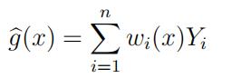
where we required that w1(x) + · · · + wn(x) = 1 for each x. However, it is often desirable for the weights {wi(x)} to satisfy other constraints. For example, if Var(εi) is very small or even 0 and g(x) is a smooth function, then we would hope that g(xi) ≈ g(xi) for i = 1, · · · , n.
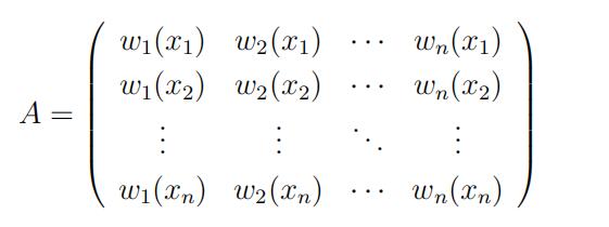
(a)Suppose that Yi= g(xi) = β0 + Σp^βkφk(xi) for i = 1, · · · , n where β0, β1, · · · , βp are some nonzero constants and φk(xi) are some functions. Define the n × n smoothing matrix
A:
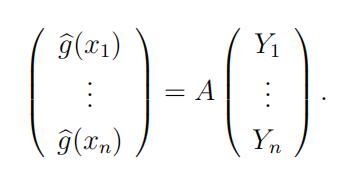
Then
If g(xi) = g(xi) for i = 1, · · · , n for all β0, β1, · · · , βp, show that statistic代写
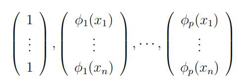
are eigenvectors of A with eigenvalues all equal to 1.
(b)A smoothing matrix A typically has a fixed number r of eigenvalues λ1, · · , λrequalto 1, with the remaining eigenvalues λr+1, · · · , λn lying in the interval (−1, 1). Usually, by varying a smoothing parameter, we can make λr+1, · · · , λn closer to 0 (which will make g(x) smoother) or closer to 1 (which can result in g(x) being very non-smooth).
If A is symmetric then A = ΓΛΓT where Λ is a diagonal matrix whose elements are the eigenvalues of A and Γ is an orthogonal matrix with Γ−1 = ΓT ; we will assume that Γ doesnot depend on the smoothing parameter (i.e. the eigenvalues of A depend on the smoothingparameter but its eigenvectors do not). In lecture, we gave the bias-variance decomposition
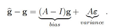
The decomposition A = ΓΛΓT make the effect of the smoothing parameter on the bias and variance components very transparent.

Show that as λr+1, · · · , λn shrink towards 0,
(i)“Aε“2= εT AT Aε decreases;
(ii)“(A−I)g“2increases if λr+1, · · , λn ≥ 0 unless g is an eigenvector of A with eigenvalue 1.
(c)In practice, the form of the smoothing matrix is typically hidden from the user and in fact, is often never explicitly computed. However, for a given smoothing procedure, we can recoverthe j-the column of the smoothing matrix by applying the smoothing procedure to pseudo-data (x1, y1∗), · · · , (xn, yn∗ ) where yj∗ = 1 and yi∗ = 0 for i j.
Consider estimating g using smoothing splines in the model
Yi = g(xi) + εi for i = 1, · · · , 20
where xi = i/21. The following R code computes the smoothing matrix A for a given value of its degrees of freedom (i.e. its trace) and then computes its eigenvalues and eigenvectors:statistic代写
> x <- c(1:20)/21
> A <- NULL
> for (i in 1:20) {
+ y <- c(rep(0,i-1),1,rep(0,20-i))
+ r <- smooth.spline(x,y,df=4)
+ A <- cbind(A,r$y)
+ }
> r <- eigen(A,symmetric=T)
> round(r$values,3)
[1] 1.000 1.000 0.913 0.579 0.262 0.115 0.055 0.029 0.016 0.010 0.006 0.004 [13] 0.003 0.002 0.002 0.001 0.001 0.001 0.001 0.001The matrix A is by definition symmetric and using the option symmetric=T in the R function eigen assures that the eigenvalues will be computed as real numbers (i.e. no imaginary component). (Note that A has 2 eigenvectors with eigenvalue equal to 1; this means that the smoothing method will recover linear functions exactly.) Repeat the procedure above using different values of df between 3 and 10. What do you notice about the eigenvalues as df varies?statistic代写
(d)The smoothing matrices in part (c) are not only symmetric but centro-symmetric; that is, if
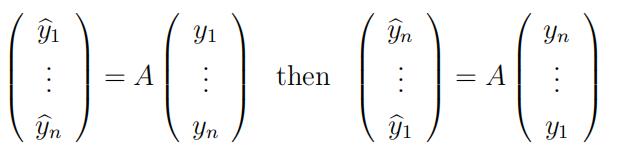
Suppose that v = (v1 v2 · · · vn)T is an eigenvector of A. Show that v is either symmetric (i.e. vj = vn−j+1 for all j) or skew-symmetric (i.e. vj = −vn−j+1 for all j).
(Hint: Define J to be the matrix that reverses the elements of a vector:
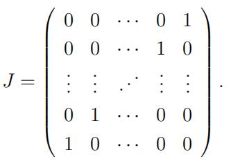
A is centro-symmetric if AJx = JAx. It suffices to show that if v is an eigenvector of A
then Jv is also an eigenvector.)
(e)(Optional but recommended) Take a look at the eigenvectors of A in part (c) (for a particular value of df). This can be done using the following Rcode:
> r <- eigen(A,symmetric=T)
> for (i in 1:20) {
+ devAskNewPage(ask = T)
+ plot(x,r$vectors[,i],type=”b”)
+ }statistic代写
(The command devAskNewPage(ask = T) prompts you to move to the next plot.) Note that the first few eigenvectors are quite smooth but become less smooth.
2.Supposethat D1, · · , Dn are random directions – we can think of these random variables as coming from a distribution on the unit statistic代写
circle {(x, y) : x2 + y2 = 1} and represent each observation as an angle so that D1, · · · , Dn come from a distribution on [0, 2π).
A simple family of distributions for these circular data is the von Mises distribution whose density on [0, 2π) is
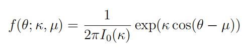
where 0 ≤ µ < 2π, κ ≥ 0, and I0(κ) is a 0-th order modified Bessel function of the first kind. In this problem, we want to derive tests of the null hypothesis H0 : κ = 0 versus the alternative H1 : κ > 0. Note that under H0, D1, · · · , Dn have a uniform distribution on the interval [0, 2π).statistic代写
(a)Suppose that we want to test H0 : κ = 0 versus H1 : κ > 0. Consider a likelihood ratio test of H0 : κ = 0 versus H0 1: κ = κ1 > 0. Show that this LR test rejects H0 : κ = 0 for large values of the statistic
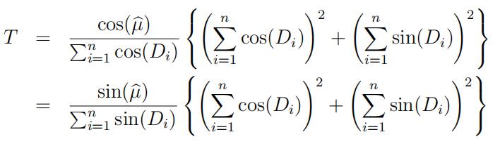
where µ is the MLE of µ (derived in Assignment #3).
(b)TheRayleigh test of H0 : κ = 0 versus H1 : κ > 0 uses a test statistic closely related to the LR statistic in part (c). Define
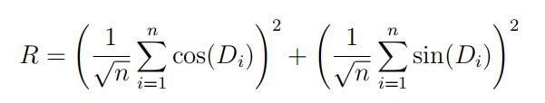
Show that the limiting distribution of R when H0 is true is Exponential with mean 1. (Hint: Use the bivariate CLT to find the joint limiting distribution of the random variables inside the parentheses.)statistic代写
(c)Atest of H0 versus H1 should be invariant under shifts of the angles D1, · · , Dn; in other words, if T = T (D1, · · · , Dn) is a test statistic for testing H0 then for any φ, T (D1, · · · , Dn) and T (D1 + φ, · · · , Dn + φ) should have the same distribution under H0. Show that this invariance condition holds for the tests in parts (a) and (b). (Hint: It’s sufficient to show that T (D1, · · · , Dn) = T (D1 + φ, · · · , Dn + φ) for any φ.)
(d)The file txt contains dance directions of 279 honey bees viewing a zenithpatch of artificially polarized light. (The data are given in degrees; you should convert them to radians.) Use the Rayleigh test to assess whether it is plausible that the directions are uniformly distributed.statistic代写
Supplemental problems (not to hand in):
3.Supposethat (X1, · · , Xn) have a joint density f (x1, · · · , xn) where f is either f0 or f1 (where both f0 and f1 have no unknown parameters).
We put a prior distribution on the possible densities {f0, f1}: π(f0) = π0 > 0 and π(f1) = π1 > 0 where π0 + π1 = 1. (This is a Bayesian formulation of the Neyman-Pearson hypothesis testing setup.)
(a)Show that the posterior distribution of {f0, f1}is
π(fk|x1, · · · , xn) = τ (x1, · · · , xn)πkfk(x1, · · · , xn) for k = 0, 1
and give the value of the normalizing constant τ (x1, · · · , xn). (Note that π(f0|x1, · · · , xn) +π(f1|x1, · · · , xn) must equal 1.)statistic代写
(b)When will π(f0|x1, · · , xn) > π(f1|x1, · · · , xn)? What effect do the prior probabilitiesπ0and π1 have?
(c)Suppose now that X1, · · , Xnare independent random variables with common density gwhere g is either g0 or g1 so that
fk(x1, · · · , xn) = gk(x1)gk(x2) × · · · × gk(xn) for k = 0, 1.If g0 is the true density of X1, · · · , Xn and π0 > 0, show that
π(f0|x1, · · · , xn) −→ 1 as n → ∞.(Hint: Look at n−1 ln(π(f0|x1, · · · , xn)/π(f1|x1, · · · , xn)) and use the WLLN.)
4.Suppose that X1, · · , Xnare independent Exponential random variables with parameter statistic代写
λ. Let X(1) < · · · < X(n) be the order statistics and define the normalized spacings
D1 = nX(1)
and Dk = (n − k + 1)(X(k) − X(k−1)) (k = 2, · · · , n).
As stated in class, D1, · · · , Dn are also independent exponential random variables with pa- rameter λ.
(a)LetX¯n be the sample mean of X1, · · , Xn and define for integers r ≥ 2
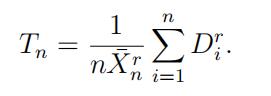
Use the Delta Method to show that √n(T − r!) −→d statistic代写
N (0, σ2(r)) where
σ2(r) = (2r)! − (r2 + 1)(r!)2
and so √n(ln(Tn) − ln(r!)) −→ N (0, σ2(r)/(r!)2).
(Hint: Note that D1 + · · · + Dn = nX¯n. You will need to find the joint limiting distribution of
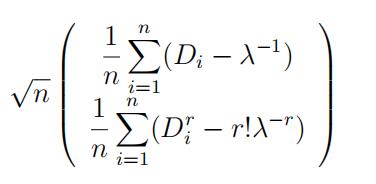
and then apply the Delta Method; a note on the Delta Method in two (or higher) dimensions can be found on Quercus. You can compute the elements of the limiting variance-covariance matrix using the fact that E(Dk) = k!/λk for k = 1, 2, 3, · · · which will allow you to computeVar(Dr) and Cov(Dr, Di).)
Note:
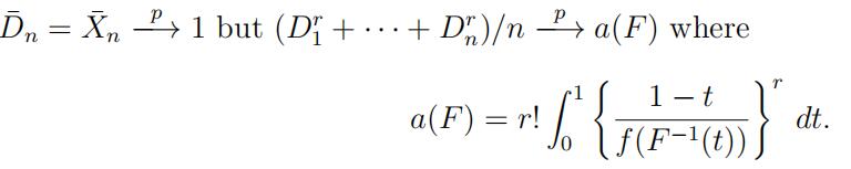
We can use the statistic Tn (or ln(Tn) for which the normal approximation is slightly better) defined in part (a) to test for exponentiality, that is, the null hypothesis that X1, · · · , Xn come from an exponential distribution; for an α-level test, we reject the null hypothesis for Tn > cα where we can approximate cα using a normal approximation to the distribution of Tn or ln(Tn). The success of this test depends on Tn −→ a(F ) where a(F ) > r! for non-exponential distributions F . Assume that the F concentrates all of its probability statistic代写
mass on the positive real line and has a density f with f (x) > 0 for all x > 0; without loss of generality, assume that the mean of F is 1. If k/n ≈ t then Dk = (n − k + 1)(X(k) − X(k−1)) is approximately exponentially distributed with mean (1 − t)/f (F −1(t)), which is constant for 0 < t < 1 if (and only if) F is an exponential distribution. Since the mean of F is 1,
By H¨older’s inequality, it follows that
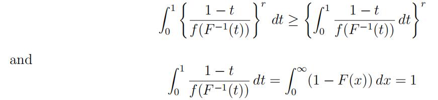
since we assume that the mean of F is 1. Thus a(F ) ≥ r!. Moreover, if a(F ) = r! then (1 − t)/f (F −1(t)) = 1 for 0 < t < 1 or (1 − F (x))/f (x) = 1 for all x > 0, which implies that F (x) = 1 − exp(−x).statistic代写
(b)Usethe test suggested in part (a) on the air conditioning data (from Assignment #1) taking r = 2 and r = 3 (using the normal approximation to ln(Tn)) to assess whether an exponential model is reasonable for these data.

其他代写:algorithm代写 analysis代写 app代写 assembly代写 assignment代写 C++代写 code代写 course代写 dataset代写 java代写 web代写 北美作业代写 编程代写 考试助攻 program代写 cs作业代写 source code代写
