Oil Forward Price Model
Oil Forward Price Model代写 To plot the forward curve for the earliest trade date and the most recent trade date in the WTI dataset
- To plot the forward curve for the earliest trade date and the most recent trade date in the WTI dataset, the first step is to do some calculations on columns: the TRADEDATE column needs to be replaced with an actual date, and a maturity column is added to the dataset.Oil Forward Price Model代写
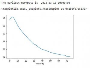
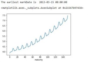
The WTI forward curve for the earliest market date:
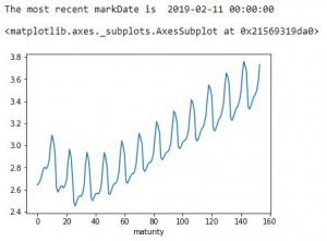
The forward curve for the last market date:Oil Forward Price Model代写
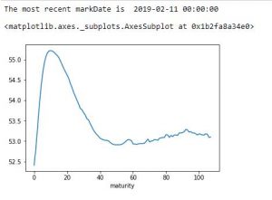
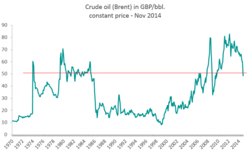
The plots indicate that the WTI curve had dropped significantly, from above 90 to around 53, during 2013 to 2019. While there was a small rebound to 55 in 2019, it decreased quickly and tended to be relatively stable later. In addition, there is no seasonality shown in the oil curve.
- To clean the data, the first step is to remove all columns with missing values. Then, compute the log return of SETTLE column and annualize the results, plot the results:
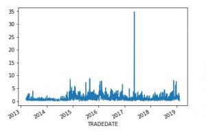
There is an obvious outlier data some time in 2017. In order to eliminate its potential adverse effect on the model, remove this offending data from the dataset.
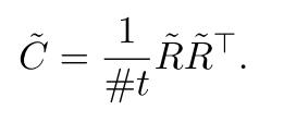
- To build volatility functions by using PCA for a 60-month oil model, the first step is to calculate covariance from log returns obtained in Q2 by formula:
Next, compute the eigenvector decomposition by formula: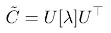
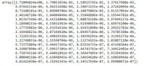
And get the amount of variance for the independent Wiener factors:
After this, define the percentage of variance explained with n factors:
![]()
- 2 factors are needed in order to explain at least 99% of the variance.
- Use 3 factors to show the three most significant volatility functions. About 99% of variance is explained by these factors. Compute the three volatility functions by formula:
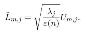
Plot the three most significant volatility functions:
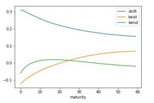
The plot shows a clear “shift”, “twist”, “bend” pattern. Values on “shift” curve have the same sign; The front end of the “twist” curve is of the opposite sign as those at the end; The “bend” curve makes the middle contracts move in a different direction than the front.
Natural Gas Forward Price ModelOil Forward Price Model代写
-
Same as what have been initially done to WTI dataset, replace an actual date with TRADEDATE, and compute the maturity column before plotting the gas forward curve.
The gas forward curve for the earliest trade date:
The forward curve for the last trade date:
The plot shows that the gas curve had a general increasing trend with a clear seasonal pattern in 2013. Between 2013 and 2019, the gas price dropped from the range of 4 to 7.5 to the range of 2.4 to 3.8. In 2019, the gas price still had the seasonally increasing pattern, and its variance for each period is clearly larger than 2013.
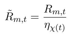
- As the previous plots show clear seasonality in the gas price, the maturities data needs to be de-seasonalized before using them to build a model. Using the first 12 months of maturities for the de-seasonalization. Compute the de-seasonalized annualized log returns by formula:
A snip of the result:Oil Forward Price Model代写
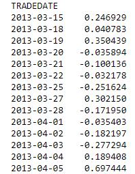
. .
. .
. .
Then, compute the seasonal factors and plot the result:
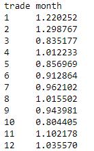
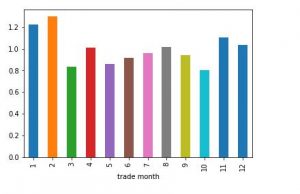
The seasonal factors show that, Nov, Dec, Jan, Feb are associated with increased volatility. This is probably beacuse that people using more gas for heat and cars during cold winter times.
- Compute the deseasonalized log returns from the seasonality factor and the log returens.
A snip of the reuslt table:
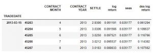
The result table indiactes that there are 144 maturities can be used to build the model
- In order to compute a PCA model for 60 maturities of gas by using the de-seasonalized annual log returns data, the first step is to define the percentage of variance explained with n factors as what have been done in WTI dataset:
![]()
The result of variances shows that 5 factors are needed to explain at least 98% of the variance. Next, using the same technique in WTI dataset, plot the three most significant volatility functions when factor=5:
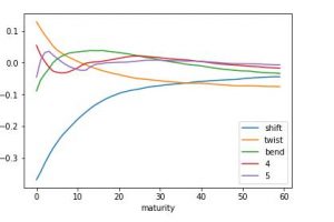
The “shift”, “twist”, and “bend” curve show expected patterns.
- Instead of using 60 maturities of gas data, de-seasonalize the log return data for the first 36 maturities. Same as the step in Q4, compute the percentage of variance explained with n factors:
![]()
This time, only 4 factors are needed to explain at least 98% of the variance.
Plot the three most significant volatility functions when factor=4:
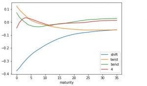
Comparing the plots for using 60 and 36 maturities data, there is no obvious difference on “shift” and “twist” curve. On the other hand, “bend” curve is smoother when using 36 maturities.

