
Research-Linked Topics: Continuous-time Linear Filter
滤波器论文代写 Your overall aim is to write a good essay about the filtering problem. You will find some possible tasks, in the form of exercises in Section 2.
1 What to do
Your overall aim is to write a good essay about the filtering problem. You will find some possible tasks, in the form of exercises in Section 2. You are not expected to complete them all. Instead they should serve as something you can focus on in your essay. 滤波器论文代写
When writing your essay do not refer to the specific exercises, your aim should be to produce something that can be read on its own. In other words do not treat this as answering an exam where you write just the solutions.
1.1 Initial 2 page part
It is recommended that you write solutions to some parts of Exercises 2.1, 2.2 and 2.3.
1.2 Main project
You should take into account the feedback received for the initial 2 page part. If the same mistakes appear uncorrected then you will certainly lose marks. It is recom- mended that you provide solutions to some of the remaining exercises. If you do less theoretical work then it is expected that you do more computational work (and that you provide careful analysis of the computational work). 滤波器论文代写
1.3 Reading
Regarding the recommended books: Bain and Crisan [1] is the most general and hence the hardest to read. Lipster and Shiryayev [4] contains many details but it may also be difficult to read. Fristedt, Jain and Krylov [2] is written very nicely at an introductory level (but may not be available in the library). Øksendal [3] is widely available and treats the linear case but differently to what was discussed in the lecture and it is not recommended.

2 Kalman–Bucy ftlter and exercises 滤波器论文代写
The continuous time linear filter is also known as the Kalman–Bucy filter. We fix a probability space (Ω, F, P), a time horizon T > 0.
The hidden “state” and “observation” processes are given as a stochastic differen- tial equation (SDE) system:
(state) dxt = Fxtdt + σdWt ,x0 ∼ N (0, r0),(observation) dyt = Hxtdt + dVt ,Y0 = 0.
Here F, H ∈ R are given constants and x0 is assumed independent of (W, V ) while (W, V ) is an R2-valued Wiener process (which in turn means that W and V are independent). 滤波器论文代写
Aim: Given a function ϕ : Rd2 → R find the best mean square estimate ϕˆ for ϕ(xt), given the observations up to time t i.e. given the path y[0,t] := (ys)s∈[0,t]. Hence we are saying that ϕˆ must satisfy:
E|ϕˆ − ϕ(xt)|2 = min E|f (y[0,t]) − ϕ(xt)|2 .
Exercise 2.1.
Show that ϕˆ = E[ϕ(xt)|σ(y[0,t])].
We now know that a conditional expectation gives the best mean square estimate but we do not know how to compute this. Let us write Yt := σ(y[0,t]) and let us define
Pt(ϕ) := E[ϕ(xt)|Yt] ∀ϕ bounded . 滤波器论文代写
Our aim is thus to be able to compute Pt for a given ϕ. Note that we may view Pt as the law of xt conditional on Yt.
Exercise 2.2.
Consider a random variable X.
i)Define the law (or distribution) ofX.
ii)Show that if we know E[ϕ(X)] for any ϕ : R → R bounded and measurable then we know the law of X. 滤波器论文代写
iii)Showthat if we know the law of X then we can evaluate E[ϕ(X)] for any ϕ : R →
R bounded and measurable. Hint: Consider simple functions ϕ first.
Exercise 2.3.
Assume that the observation process is replaced by dyt = dVt. That is, the observations do not tell us anything about the process. Assume that ϕ ∈ C2.
- Show that Pt(ϕ) = E[ϕ(xt)].
- Use Itˆo formula and then take expectation to show that
dPt(ϕ) = Pt(Lϕ)dt, 滤波器论文代写
where L(x)ϕ(x) := 1σ2ϕ′′(x) + Fxϕ′(x).
3.Comment on this
Proposition 2.4 (Kalman–Bucy Filter). For the linear filtering problem here we have that Pt, which is the distribution of xt conditional on Yt is normal with conditional mean xˆt and conditional variance Rt, where
dxˆt = F xˆtdt + HRtd(yt − Hxˆtdt) ,
and Rt satisfies the ordinary differential equation (ODE) 滤波器论文代写
xˆ0 =0
dRt = σ2 + 2FR dt t
− H Rt , R0
= r0 .
Note that ODEs of this form are called Riccati equations.
Exercise 2.5.
Prove the first statement of Proposition 2.4. That is, show that Pt, which is the distribution of xt conditional on Yt is normal. Hint. There is a Lemma in Bain and Crisan [1] that makes a good starting point but you should include more detail e.g. by following the reference given there. 滤波器论文代写
Exercise 2.6.
Show that we have the equations for xˆt and Rt as claimed in Proposi- tion 2.4. You can do this by considering
(state) dxt = b(xt, yt)dt + θ(xt, yt)dwt + ρ(xt, yt)dvt , x0 = ξ,
(observation) dyt = B(xt, yt)dt + dvt ,
Y0 = η .
Here xt ∈ Rd1 , yt ∈ Rd2 , (w, v) is a Rd′+d2 -Wiener process (in particular all components are independnt and so w and v are independent Wiener processes taking values in Rd and Rd′ respectively). The initial points (ξ, η) are assumed independent of each other and (w, v). The functions 滤波器论文代写
b : Rd1+d2 → Rd1 , B : Rd1+d2 → Rd2 ,
θ : Rd1+d2 → Rd1×d′, ρ : Rd1+d2 → Rd1×d2,
are assumed to be Lipschitz continuous.
Now follow these steps:
i)Let
to define a change of measure P¯ and use Girsanov’s theorem to show that yt − y0
is a Wiener process (assume B is bounded).
ii)Use Lemma 3.1 to show that with µt(ϕ) := E¯[ϕ(xt)γt−1|Yt] we have
P (ϕ) = µt(ϕ) . 滤波器论文代写
t µt(1)
iii)Derive the Zakaiequation:
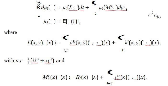
Hint: You can use Lemma 3.3 without proof.
iv)Derive the Kushner–Shiryayevequation:
dPt(ϕ) = Pt(Ltϕ)dt + (Pt(Mtϕ) − Pt(ϕ)Pt(Bt)) dV¯t , P0(ϕ) = E[ϕ(ξ)],
∀ϕ ∈ C2 . (1) 滤波器论文代写
Here dV¯t := dyt − Pt(Bt)dt. This is called the “innovation process”.
Hint: First show that dµt(1) = µt(1)Pt(B)dyt by using Lemma 3.3 again.
v)UseExercise 5 and apply (1) with ϕ(x) = x and ϕ(x) = x2 to obtain the result of Proposition 2.4.
vi)Explainwhy using ϕ(x) = x (or x2) is not mathematically valid and suggest how you could overcome this.
Exercise 2.7.
Use a programming language of your choice (though Matlab, Python or R would probably be the most suitable) to implement the Kalman–Bucy filter. You will need to carry out the following steps: fix T > 0, and N ∈ N for the number of time steps you will use in discretization. Let τ = T/N .
i)Simulate the stateas
Xi+1 = Xi + FXiτ + σ√τ Zi , i = 0, . . . , N − 1.
Here Zi are independent samples from N (0, 1) (and independent from X0).
ii)Simulate the signalas 滤波器论文代写
Y i+1 = Y i + HXiτ + √τ Z˜i , i = 0, . . . , N − 1.
Here Z˜i are independent samples from N (0, 1) (and independent from X0 and from Zi).
iii)0Solve the Riccati ODE
iv)Calculate xˆ from the above.
You should be able to produce simulation results similar to Figure 1.
3 Additional Material 滤波器论文代写
We will need a Lemma on conditional expectations under a change of measure:
Lemma 3.1. Take two probability measures P and P¯ such that1 P¯ << P with
dP¯ = ΛdP. 滤波器论文代写
Let G be a sub–σ–algebra of F. Then P¯ almost surely E[Λ|G] > 0. Moreover for any
F-random variable X we have
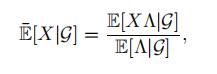
where E¯ denotes expectation taken under P¯.
1Recall that we say that a measure P¯ is absolutely continuous with respect to a measure P if P(E) = 0 implies that P¯(E) = 0. We write P¯ << P.
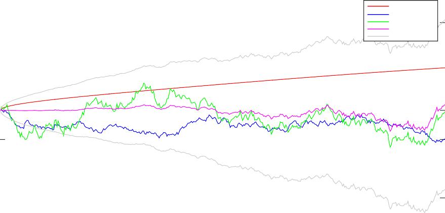
Figure 1: Example of one run of the Kalman–Bucy filter from solution to Exercise 2.7. Note that the parameters taken were σ = 0.5, F = 1, r0 = 10−5, H = 3/2, T = 1, N = 400.
Exercise 3.2.
Prove Lemma 3.1.
We also require the following Lemma, which we present without proof.
Lemma 3.3. Fix a probability space (Ω, F, P¯). Let (W, Y ) be a d′ + d2–dimensional Wiener process. Let ξ, η be random variables independent of (W, Y ) and let Yt := σ(η, Ys : s ≤ t). Let (ft)t≤T be a bounded stochastic process. Then 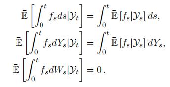
References 滤波器论文代写
[1]Bain and D. Crisan. Fundamentals of Stochastic Filtering. Springer, 2009. [2]Fristedt and N. Jain and N. V. Krylov. Filtering and Prediction: A Primer. AMS,2007. [3]Øksendal. Stochastic Differential Equations. Springer 2003. [4]S. Lipster and A. N. Shiryayev. Statistics of Random Processes. Springer, 2001.
其他代写:代写CS C++代写 java代写 matlab代写 web代写 app代写 作业代写 物理代写 数学代写 考试助攻 paper代写 金融经济统计代写 python代写 Exercise代写
