machine learning algorithms代写 Coursework代写 exercises代写

COMP3223: Coursework

machine learning algorithms代写 1Due dateThe hand-in date for the assignment is Wednesday, November 27, 2019 .2IntroductionThe exercises are meant to help you

1 Due date machine learning algorithms代写

The hand-in date for the assignment is Wednesday, November 27, 2019 .

2 Introduction machine learning algorithms代写

The exercises are meant to help you understand the course material in depth. You will find that using tools such as scikit-learn, which are there for you to use in practical contexts, will make the task of completing your coursework much simpler. However, for developing a thorough understanding of those implementations you will need to explore how the data gets transformed using mathematical methods, and you need to implement the algorithms yourself. You may use the scikit-learn libraries to check your implementations if you wish. However, for many of the data preparation steps such as loading, split- ting data into training and test tests randomly and so on, you can use canned routines such as those in scikit-learn. For some tasks I have also given you pieces of code that you can reuse, and you can repurpose the jupyter lab note- books as well.machine learning algorithms代写

A useful blog for many of the machine learning algorithms you will en- counter in the module is at https://jermwatt.github.io/mlrefined/index. html based on the book [5]. There are umpteen references on the web you may wish to consult. However, for most of the exercises [2] and [3] should give you food for thought and influence the way you write your report.

Some of you may wish to work on other datasets for more challenging tasks than those required of you here. Here are a couple of sources:

1. https://www.kaggle.com
2. https://archive.ics.uci.edu/ml/datasets.php

3 Submission guidelines machine learning algorithms代写

The report should focus on the key conceptual steps that underpin each al- gorithm, illustrating your understanding by pointing to the results you obtain that should be summarised in graphical or tabular form. Some of these are asked for explicitly in the questions below, others are left to your judgement. All else being the same, a well articulated report that shows evidence of depth of understanding will get a higher mark than one where the same results are de- scribed, but less cogently. There are page limits signposted in some of the sec- tions and the other sections should merit a similar allocation of space. These limits are not going to be policed rigorously but are intended as a guide for you to gauge how much is too much or too little. There will be a handin page for you to submit a report and code files.

4 Linear Regression with non-linear functions

[4 marks]

In this exercise you have to perform the task of fitting polynomial func- tions to y(x) = sin(4πx) + ϵ where ϵ is a noise term. You have to generate a number N of points chosen randomly from 0 ⩽ x ⩽ 1. Your training and test sets will be taken from these (x_n, y_n) pairs, for n = 1, . . . , N.machine learning algorithms代写

rn = np.random.uniform(0, 1, n)

x = np.reshape(np.sort(rn, axis=0), (n, 1))

4.1 Performing linear regression with polynomials and radial basis functions

In this part you will model each (input, target) pair (t_n, x_n) by a linear com- bination of basis functions: y(x; w) = j w_jϕ_j(x). You will take two classes of functions ϕ_j(x) for your basis elements to fit the training and test data sets that you generate:

1. polynomials:ϕ_j(x_n) = x^{j machine learning algorithms代写}

where x_n is an input value.

2. Gaussianradial basis functions (RBF): for each training input x_n,

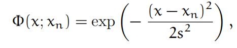
and ϕ_j(x_n) = Φ(x_j; x_n) for 0 ⩽ x_j ⩽ 1, j = 1, . . . , p.

1.Constructa design matrix A by concatenating to a column of ones p

columns ϕ₁(x_n), . . . , ϕ_p(x_n). The column entries are ϕ_j(x_n), n = 1, . . . , N.

def gaussian_basis_fn(x, mu, sigma=0.1):

return np.exp(-0.5 * (x - mu) ** 2 / sigma ** 2)

def polynomial_basis_fn(x, degree): return x ** degree

def make_design(x, basisfn, basisfn_locs=None): if basisfn_locs is None:

return np.concatenate([np.ones(x.shape), basisfn(x)], axis=1) else:

return np.concatenate([np.ones(x.shape)] + \ [basisfn(x, loc) for loc in basisfn_locs], axis=1)

2. The weights that minimise the lossfunction

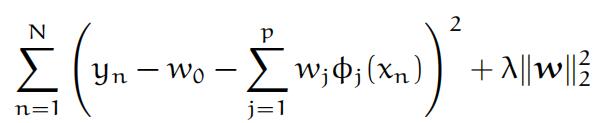
are given by the analytical expression¹

w =  (A^T A + λI_p+1)⁻¹A^T y, (1)

where I_m stands for a m × m identity matrix².

4.2 How does regression generalise? Computing bias and variance

[4 marks]

1You should know how to derive it.machine learning algorithms代写

2An alternative expression is w = A^T (AA^T + λI_N)⁻¹y

This section gets you to explore the models learned by linear regression, by looking at the dependence of the optimal weights on training data and the scale of regularisation. When writing up the results of this section about the ability of the models to generalise using the tasks below, try to relate the weights from eq.(1) to your analysis.machine learning algorithms代写

1.Split up your data into a training S^trand test set S^ts and measure the mean of the squared residuals

on the test set S^ts as a performance metric for each model. Plot this measure as a function of: (1) the number of basis components ϕ_j ; (2) the strength of the regularisation coefficient λ. You could call

from sklearn.model_selection import train_test_split

and look up the function description of train_test_split.machine learning algorithms代写

2. Samplefrom your training set S^tr to create B (potentially overlapping) data-sets of smaller cardinality S_i to train  (This is similar to what you did in Lab 2, where you trained on 1000 datasets each of two different sizes.)  S_i  ⊂ S^tr and |S_i|/|S^tr|  =  r some ratio of your choice.  Training

a regression model with p + 1 weights on a dataset S_i gives rise to a

model f(x; w_i) (now indexed by the data set on which it is trained) with a corresponding loss L_i on your test set, i = 1, . . . , B, a number that you can compute. The distribution of these B losses contributes to the evaluation of the learning model in terms of bias and variance, which you should quantify. Evaluate the bias and variance of these two classes of function approximations for a few choices of p. Again, the choices of p values should be chosen to illustrate observable differences.

5 Classification

You will explore two methods for some toy datasets in order to get familiar with some of the issues to do with projections and data transformations. You will generate one of the two datasets yourself using a random number genera- tor. The other is an old classic – Ronald Fisher’s Iris dataset that can be loaded using scikit-learn’s data loader.machine learning algorithms代写

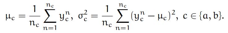
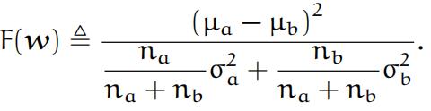
You will first explore Fisher’s LDA for binary classification for class labels aand b. In Fisher’s method a direction defined by vector w = w1w₂) is chosenso that the data xⁿ projected on to w maximises the separation between the a and b type distributions. (n is a data index, ranging from 1 to n_a for class a, and from 1 to n_b for class b, here used in superscript; it is not the n-th power of x.) Setting yⁿ ≜ w · xⁿ for class label c ∈ {a, b} the scalar means and

standard deviations of the projected data become

The direction w is chosen in order to maximise the Fisher ratio F(w): Fisher

ratio

5.1 Data 1: separate 2 Gaussians

The data for this part are to be generated by you. Generate data from two 2-dimensional Gaussian distributions

x_a ∼ N(x|m_a, S_a),  x_b ∼ N(x|m_b, S_b)

where m_a, m_b are the (2 × 1) mean vectors and S_a and S_b are the (2 × 2)

covariance matrices that define normal distributions. Let the number of data

points from each type a, b be n_a and n_b. If the classes are widely separated or if they overlap significantly it will be hard for you to explore and demonstrate the consequences of choosing different directions, and thus learn from the experience. Hence, make the differences of the means of the order of magni- tude of the standard deviations. The precise values will affect the results of the following tasks and you can experiment with numerical values that help you appreciate the pros and cons of the classification method. This will determine the evidence you provide in the report that demonstrate your insights on the nature of the learning algorithm.machine learning algorithms代写

The following tasks are broken up into two chunks to demarcate bow the marks are to be allotted, even though they are all connected. You will write up your observations in no more than 2 pages, providing evidence based on your experiments,and discuss what you have learned. You should read Section 4.4 of [4] (or Section 4.3of [3]) for guidance and ideas.

1.Thispart is for visual exploration of the consequences of projecting data onto a lower dimension.[3 marks]

(a)Make afew (between 2 − 4) illustrative choices for the directionw and plot the histograms of the values yⁿ and yⁿ.  You shoulda bmake choices that make a difference to the nature of the resulting histograms.machine learning algorithms代写

(b)Plot the dependence of F(w) on the direction of w byrotating The expression

some random starting weight vector w(0) = (w₁, w₂)^T

ing it by angles θ to get w(θ) = R(θ)w(0) where

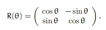
provided in the introduction to the Classification section.

Find the maximum value of F(w(θ)) and the corresponding direc-

tion w^∗:

Aside: In the lectures you will have come across the idea of change of basis using orthogonal transformations, for instance, using sets of orthogonal eigenvectors/singular vectors. The columns of the matrix R(θ) are orthogonal.

2.Thispart makes you look at probability distributions visually by drawing contour plots and/or histograms.[4 marks]

(a)Sincethe generating distributions for the classes are known, plot the equi-probable contour lines for each class and draw the direc- tion of the optimal choice vector w.machine learning algorithms代写

(b)Use Bayes’ theorem to write down the logarithm of the ratio of conditional probabilities (calledlog-odds)

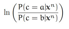
and plot the decision boundary where this quantity vanishes. In other words, for each point x ∈ R2 check whether the log-odds is positive, negative or zero. The decision boundary is the set of points where the log-odds vanishes.

• Plotthe decision boundary for both S_a = S_b and S_a ̸= S_b.machine learning algorithms代写

5.2 Data 2: Iris data

[5 marks]

In this section you will perform the same LDA task on the famous Iris dataset https://en.wikipedia.org/wiki/Iris_flower_data_set which can be downloaded from http://archive.ics.uci.edu/ml/datasets/Iris. While the previous exercise was done by finding the weight vector to project on by direct search, here you follow Fisher and solve the generalised eigenvalue con- dition for optimal weights.machine learning algorithms代写

With more features and classes, you will need to compute the between- class and within-class variance-covariance matrices Σ_B and Σ_W:

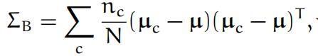where µ is the mean of class means,

and Σ_W is the sum of the covariance matrices for each class. n_c is the number of data samples in class c and N = c n_c. In case there are different numbers of training data points from each class, you have to scale any class dependence by the corresponding fraction of class members in the population. (In the Iris data set all three classes have 50 members, so you can skip this step.)

2.Find the optimal direction w^∗for projecting the data onto.

You will need to solve the generalised eigenvalue problem Σ_Bw = λΣ_Ww. Sec- tion 2, 16.3 of [1] and eq. (4.15) of [3] has further details.machine learning algorithms代写

Suggestions: The standard libraries in scipy (and others) can give you the gen- eralised eigenvalues and eigenvectors. Since the covariance matrix is symmetric, the function you should call in numpy/scipy is eigh, and not eig, although for problems of this scale it won’t make a difference and you can eyeball the eigenval- ues. In particular, the eigenvalues returned by eigh are sorted. You must also check the answer provided by verifying that the generalised eigenvalue condition Σ_Bw = λΣ_Ww holds. This will clarify the notational conventions of the soft- ware used. Sometimes it is the transpose of the returned matrix of vectors thatcontains the eigenvectors, so please make sure you understand what is being re- turned. You should also discover that the rank of Σ_B is limited by the number of

classes. Rank condition

2. Displaythe histograms of the three classes in the reduced dimensional space defined by w^∗.
3. Presentyour results with reflections and evidence in no more than 2 pages. You need to discuss the relation between the class separation task and the generalised eigenvector formulation taking into account the question in the last  You should comment on how this method com- pares with the method in the 2-gaussian separation exercise above.

References

• Barber. Bayesian Reasoning and Machine Learning. Cambridge University Press, 04-2011 edition,2011.
• Christopher Bishop. Pattern Recognition and Machine Learning. Springer, 2006.
• TrevorHastie, Robert Tibshirani, and Jerome  The Elements of Statistical Learning. Springer Series in Statistics. Springer New York Inc., New York, NY, USA, 2nd edition, 2009. machine learning algorithms代写
• GarethJames, Daniela Witten, Trevor Hastie, and Robert  An Introduction to Statistical Learning: With Applications in R. Springer Publish- ing Company, Incorporated, 2014.
• JeremyWatt, Reza Borhani, and Aggelos  Katsaggelos. Machine Learn- ing Refined: Foundations, Algorithms, and Applications. Cambridge University Press, 2016.

其他代写：考试助攻 计算机代写 作业帮助 assembly代写 function代写 paper代写 金融经济统计代写 web代写 编程代写 report代写 数学代写 finance代写 python代写 java代写 code代写 代码代写 algorithm代写

合作平台：天才代写 幽灵代写 写手招聘 Essay代写