
Time series forecasting for NN5-041 and NN5-096
Time series forecasting代写 e build three types of models of forecasting, namely exponential smoothing, ARIMA, and time series regressions
Executive summary Time series forecasting代写
We build three types of models of forecasting, namely exponential smoothing, ARIMA, and time series regressions for two time series, NN5-041 and NN5-096 respectively, and test their performance over the naïve and seasonal naïve methods for in-sample goodness of fit.

We find that for NN5-041, i)
exponential smoothing with additive errors, no trends and additive seasonality is best in its class; ii) ARIMA (0, 1, 1) with seasonality = 7 performs better than other ARIMA models; and iii) time series regression with 1 lag and 6 seasonality dummies is the simplest yet informative regression models among our three candidate. And we compare the above three models with the benchmark model of naïve and seasonal naïve models and find that the time series regression model performs the best in terms of less MSE, MAE, and MPAE. So, we choose this one to give out-of-sample forecast for 14 observations.
For NN5-096, we find that: i) exponential smoothing with additive errors, no trends and additive seasonality is best in its class; ii) ARIMA (1, 1, 0) with seasonality = 7 performs better than other ARIMA models; and iii) time series regression with 3 lag and 6 seasonality dummies is the simplest yet informative regression models among our three candidate. And we compare the above three models with the benchmark model of naïve and seasonal naïve models and find that the time series regression model performs the best in terms of less MSE, MAE, and MPAE. So, we choose this one to give out-of-sample forecast for 14 observations.
1. Introduction
In this project we apply various estimation and forecasting methods on two times series, namely NN5-041 and NN5-096 to figure out which one performs best in terms of in-sample goodness of fit, measured by indicators such as ME, MSE, and MAPE. These methods include three groups, namely exponential smoothing, ARIMA models, and time series regression and we consider several potential settings for each group. We use the naïve and seasonal naïve method as benchmark, and compare their performance based on the above-mentioned measures. Once we select the best model, we conduct out-of-sample prediction of 14 values for 2 weeks.
The results from our analysis are as follows.
First, for time series NN5-041, we find that: i) exponential smoothing with additive errors, no trends and additive seasonality is best in its class; ii) ARIMA (0, 1, 1) with seasonality = 7 performs better than other ARIMA models; and iii) time series regression with 1 lag and 6 seasonality dummies is the simplest yet informative regression models among our three candidate. And we compare the above three models with the benchmark model of naïve and seasonal naïve models and find that the time series regression model performs the best in terms of less MSE, MAE, and MPAE. So, we choose this one to give out-of-sample forecast for 14 observations.
For NN5-096, we find that: i) Time series forecasting代写
exponential smoothing with additive errors, no trends and additive seasonality is best in its class; ii) ARIMA (1, 1, 0) with seasonality = 7 performs better than other ARIMA models; and iii) time series regression with 3 lag and 6 seasonality dummies is the simplest yet informative regression models among our three candidate. And we compare the above three models with the benchmark model of naïve and seasonal naïve models and find that the time series regression model performs the best in terms of less MSE, MAE, and MPAE. So, we choose this one to give out-of-sample forecast for 14 observations.
The following sections are organized as follows: we conduct some descriptive analysis in section 2, where trend, seasonality and irregular terms are decomposed for two series. In section 3, we fit the above three models along with the benchmark naïve model and compare their performance for two series separately. The out-of-sample forecast is available after picking out the best model, i.e., linear regression with 1 lag and 6 seasonal dummies.
2. Descriptive analysis
First, we need get a rough idea of how our data looks like by conducting descriptive statistic analysis. Our data begins on Mar 18, 1996 and ends on Mar 22, 1998 and are reported daily. They are plotted as follows:
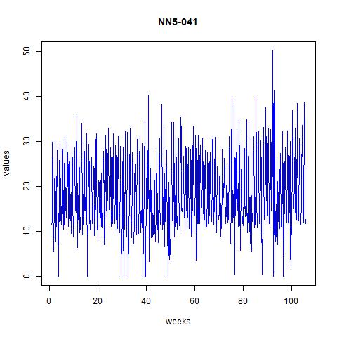
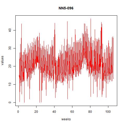
Figure 1 time series plot for NN5-041 and NN5-096
From the above plots we can see that there are some seasonality and trend across time. However, the order of seasonality is hard to find from the massive data we plotted there. Hence, we plot them for up to 50 days in the next two figures:
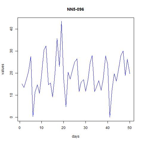
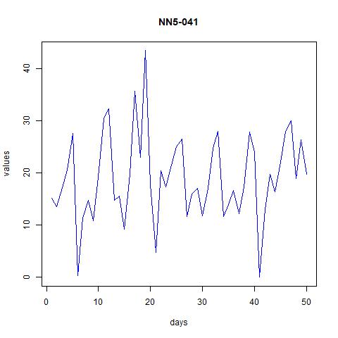
Figure 2 time series plot for NN5-041 and NN5-096 (first 50 observations)
From these figures it seems that the data might have weekly patterns, i.e., frequency=7.
We also confirm this from the seasonal plots:
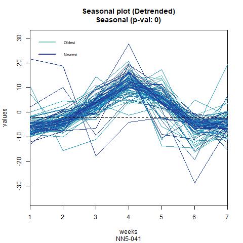
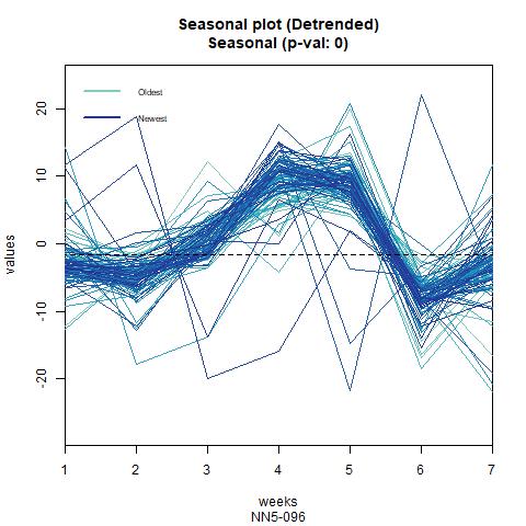
Figure 3 Seasonal plot for NN5-041 and NN5-096 (frequency=7)
In next page, we further decompose the seasonality and trend terms, where multiplicative decomposition is selected (additive decomposition gives similar results, see appendix for details). For both series, the seasonality term is very strong, while the trend term seems to fluctuation around 20. The irregular term, i.e., the residuals is centered around zero and exhibit huge variance in certain periods.

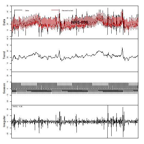
Figure 4 Trend and Season decomposition of NN5-041 and NN5-096 (assuming multiplicative decomposition)
3. Estimation and prediction Time series forecasting代写
In this section we report the results for various estimation and prediction methods. We use naïve and seasonal naïve methods as benchmark and compare the in-sample performance our three types of models based on indicators such as ME, MSE, and MAPE. Our selection process is divided into two steps: first, for several possible settings under one group of models, we pick the best performing one based on these indicators; second, we compare these candidate models with each other as well as with the benchmark models of naïve and seasonal naïve methods. Finally, we use the chosen model to generate out-of-sample prediction for 14 days (i.e., 2 weeks). Since the procedure is exactly the same for two series, we detail them in section 3.1. for NN5-041 and only report the results in section 3.2. for NN5-096.
3.1. Time series NN5-041
3.1.1. Naïve and seasonal naïve methods as benchmark
Now, lets fit our data with some simple methods and see how they performs. The easiest and most intuitive one to implement is the naïve method. The resulting fitted values are plotted against the original values in the left panel. Note that we can also include seasonal terms in the naïve model, which is depicted in the right panel.

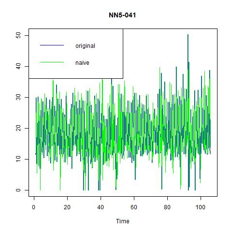
Figure 5 naïve and seasonal naïve methods for NN5-041
We report the performances of these two methods applied to our two series in the next table:
Table 1 Performance indicators for naïve and seasonal naïve methods for NN5-041
Naïve
Seasonal naïve
ME
0.0002
0.0730
MSE
76.3389
42.8965
RMSE
8.7372
6.5495
MAE
6.8508
4.2702
MAPE
61.6955
46.0497
So, the naïve method gives the lower ME, but higher MSE, RMSE, MAE, and MAPE than seasonal naïve method. This is because by including a seasonality term, the later one can achieve higher prediction power but might be a little bit biased.
3.1.2. Exponential smoothing
We consider three exponential smoothing models in this section, namely fixed alpha = 0.15, optimal alpha, and ZZZ which automatically builds the “optimal” exponential smoothing models. The fitted values are plotted in the following figures:
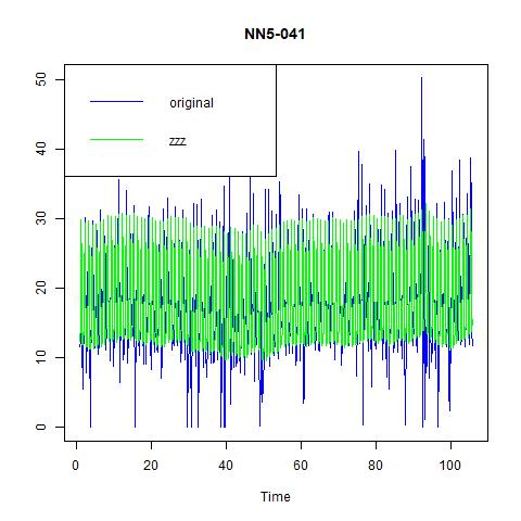
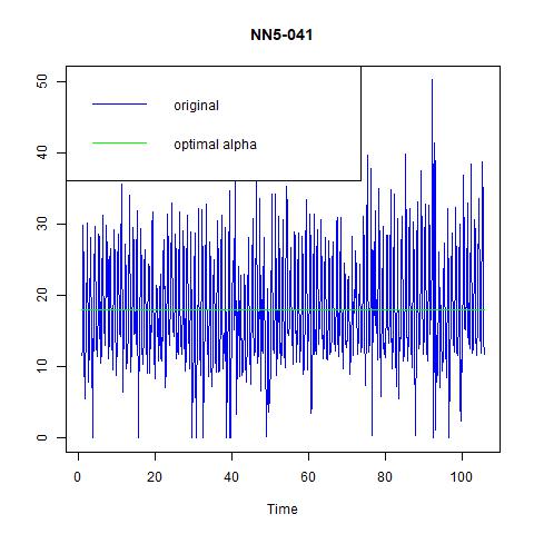
Figure 6 three exponential smoothing methods for NN5-041
From these three figures, we find that: i) alpha=0.15 does not capture the high volatility in the data; ii) optimal choice of alpha under ANN simple gives us a constant estimate of the series, hence very pool prediction power; and iii) the optimal method chosen by the program is ANA, i.e., additive errors, no trend, and additive seasonality. And from the following table on the performance, we find that the third one, ANA performs the best among three models.
Table 2 Performance indicators for three exponential smoothing methods for NN5-041
Alpha=0.15
Optimal alpha ANN
ZZZ=ANA
ME
0.0481
0.0068
0.0814
MSE
69.3752
63.4995
23.7625
RMSE
8.3292
7.9687
4.8747
MAE
6.8973
6.5929
3.1989
MAPE
81.0178
80.6679
50.5366
3.1.3. ARIMA model
In order to apply the ARIMA model, we should first test whether the series are stationary, which can be done through the KPSS test and ADF test. The results for NN5-041 are: i) the KPSS level = 0.54047 with truncation lag parameter = 6 and p-value = 0.03255; ii) the ADF test statistic = -7.5719, with lag order = 9 and p-value = 0.01.Time series forecasting代写
Note that the null hypothesis for KPSS test is that the series are stationary while the null for ADF test is that there exists a unit root in the time series. The controversial conclusions of these two tests suggest that for concreteness, we should take first difference and consider the impact of seasonality. To make it clear, we plot the ACF and PACF figures in figure 7 for the original series as well as the series after first difference and with lag =7 in the next page.
From the PACF plot, we can set the AR order to be 1. And the ACF plot does not exhibit significant peaks other than at 1 and numbers 7, hence we could set up an ARIMA (1, 1, 0) model with seasonality = 7. The resulting fitted values as well as residuals are plotted in figure 8. Finally, we also let the program to automatically decide which ARIMA model to use,
and the results for that automized ARIMA are reported in figure 9.
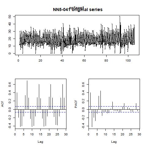
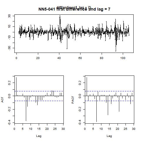
Figure 7 ACF and PACF for the original series and the first differenced series with lag = 7 for NN5-041
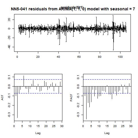
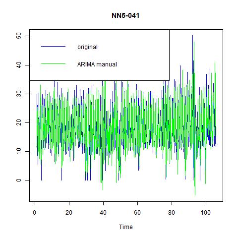
Figure 8 fitted values and residuals from ARIMA (1, 1, 0) model with seasonality = 7 for NN5-041
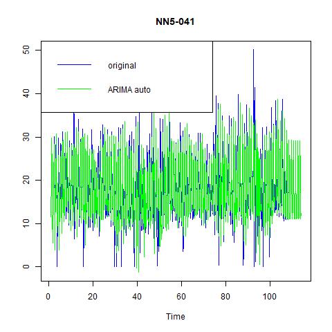
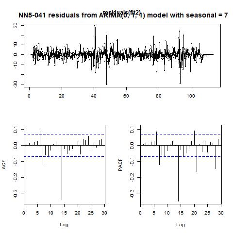
Figure 9 fitted values and residuals from automatically selected ARIMA model with seasonality = 7 for NN5-041
Table 3 Performance indicators for two ARIMA models for NN5-041
ARIMA (1, 1, 0) with seasonal = 7
ARIMA (0, 1, 1) with seasonal = 7
ME
-0.0005
-0.0008
MSE
33.9486
29.5814
RMSE
5.8265
5.4389
MAE
3.9269
3.6531
MAPE
45.0774
47.8491
Comparing the performance of our manually selected and the automatically chosen models, we find that the later one performs better in terms of MSE (hence RMSE) and MAE, but slightly worse in terms of MAPE. From the figures we also find that the later one could fit the highly volatile profile of the data quite well. Hence, we would prefer it over the former one, and choose it as the candidate for the final comparison.Time series forecasting代写
3.1.4. Time series regression
Now, let’s consider a linear regression approach. Note that we have several candidate variables for time series regression: the lagged values for our variable of interests, the seasonality variables, as well as another variable, i.e., NN5-096. We report the coefficient estimates for three manually set regression models in table 4, their fitted values against observed values in figure 10, and performance indicators in table 5.
Table 4 Regression coefficients for three models for NN5-041
(1)
(2)
(3)
Intercept
10.5964
12.9677
8.3001
(0.6601)
(1.4657)
(1.4703)
1lag
0.2354
0.2579
0.2124
(0.0378)
(0.0397)
(0.0378)
2lag
-0.1189
-0.1177
(0.0412)
(0.0390)
3lag
0.0097
-0.0041
(0.0408)
(0.0386)
NN5-096
0.3063
(0.0321)
Seasonality dummy
Yes
Yes
Yes
Adjusted R-squared
0.6498
0.6557
0.6947
Note: standard errors are in bracket.
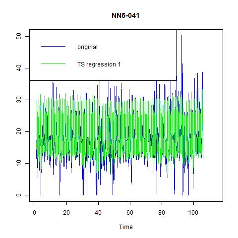
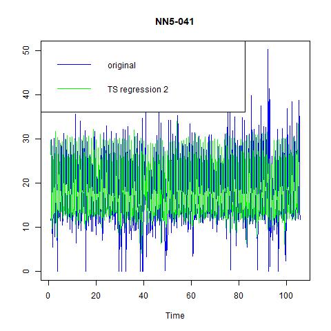
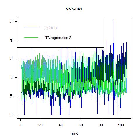
Figure 10 fitted values for three time series regression models for NN5-041
Table 5 Performance indicators for three linear regression models for NN5-041
Model (1)
Model (2)
Model (3)
ME
0.0000
0.0000
0.0000
MSE
22.0707
21.7208
19.3060
RMSE
4.6979
4.6606
4.3938
MAE
3.0146
3.0347
2.9791
MAPE
21.2463
23.2725
23.8383
From the above tables and figures, we can see that although the inclusion of more variables in model (2) and model (3) has increases the adjusted R-squared, but the improvement is not significant. More importantly, in terms of in-sample performance, model (1) has the lowest MAPE, while the gap in other indicators with model (2) and model (3) are also negligible. Hence, we would like to choose model (1), the simplest yet informative one as our candidate model. In fact, it is just an AR (1) model with six seasonality dummies (because seasonal = 7).
3.1.5. Comparison and forecasting
Now we have several candidate models: ES with ANA, ARIMA (0, 1, 1) with seasonal = 7, and linear regression with 1 lag and 6 seasonality dummies. Comparing them with each other as well as with the naïve and seasonal naïve models tells us that the linear regression model performs the best: it has zero ME; lowest MSE, MAE, and MPAE. Hence, we would choose this one and forecast 14 out-of-sample observations. The results are:
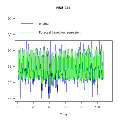
Figure 11 Forecast based on regression with 1 lag and 6 seasonal dummies for NN5-041
3.2. Time series NN5-096
3.2.1. Naïve and seasonal naïve methods as benchmark
We still fit naïve methods as benchmark, and find that including seasonality can substantially improve the prediction power:
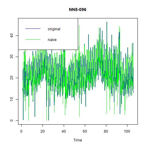

Figure 12 naïve and seasonal naïve methods for NN5-096
Table 6 Performance indicators for naïve and seasonal naïve methods for NN5-096
Naïve
Seasonal naïve
ME
-0.0027
0.0730
MSE
96.8614
42.8965
RMSE
9.8418
6.5495
MAE
7.3105
4.2702
MAPE
86.6312
42.7537
3.2.2. Exponential smoothing
The fitted values for three ES methods are plotted in next page; their performance is in table 7. It is clear that exponential smoothing with additive error, no trend, and additive seasonality still works best for our model.
Table 7 Performance indicators for three ES methods for NN5-096
Alpha=0.15
Optimal alpha
ZZZ = ANA
ME
0.0434
0.0720
0.0350
MSE
67.4077
64.2901
25.0004
RMSE
8.2102
8.0181
5.0000
MAE
6.5936
6.4561
3.0614
MAPE
71.7674
70.4082
40.8222
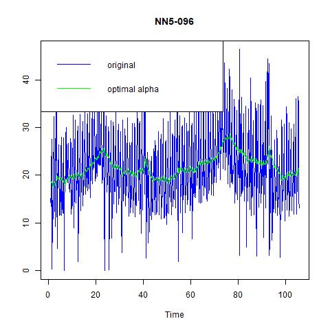
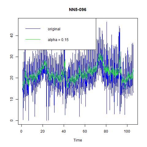
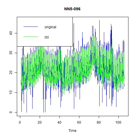
Figure 13 three exponential smoothing methods for NN5-096
3.2.3. ARIMA model
The results of KPSS and ADF test for for NN5-096 are: i) the KPSS level = 0.8183 with truncation lag parameter = 6 and p-value = 0.01; ii) the ADF test statistic = -5.4515, with lag order = 9 and p-value = 0.01. The ACF and PACF curves for the original and the first-differenced series with lag=7 are reported in figure 14. We choose the ARIMA (0, 1, 1) model with seasonal = 7 manually. And the model chosen by the program is ARIMA (1, 1, 0) with seasonal = 7. And the auto-generated model has better performance than our choice in terms of MSE, MAE, and MAPE. And the small difference in ME does not matter for its dominance.
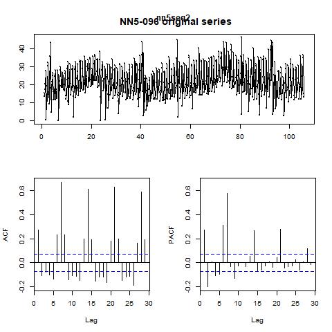
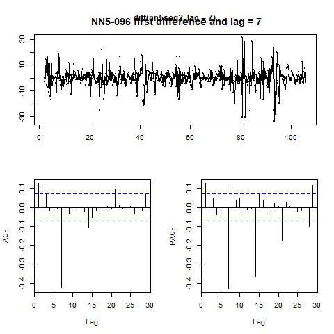
Figure 14 ACF and PACF for the original series and the first differenced series with lag = 7 for NN5-096
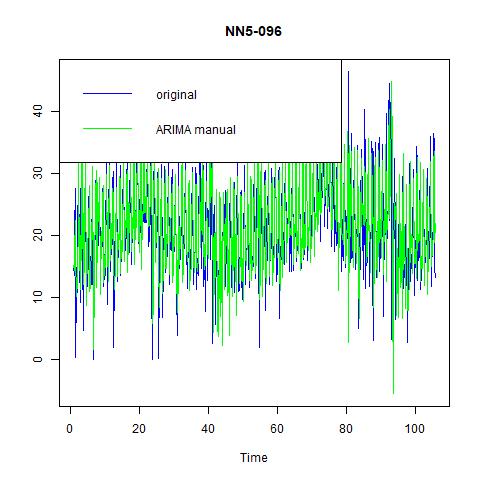
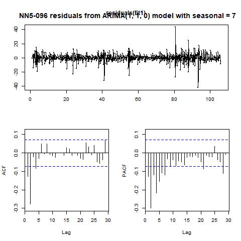
Figure 15 fitted values and residuals from ARIMA (0, 1, 1) model with seasonality = 7 for NN5-096
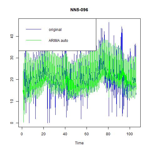
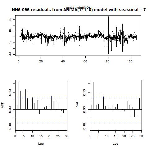
Figure 16 fitted values and residuals from automatically selected ARIMA model with seasonality = 7 for NN5-096
Table 3 Performance indicators for two ARIMA models for NN5-041
ARIMA (0, 1, 1) with seasonal = 7
ARIMA (1, 1, 0) with seasonal = 7
ME
-0.0047
0.0649
MSE
34.7334
26.9093
RMSE
5.8935
5.1874
MAE
3.8979
3.4441
MAPE
49.1434
37.7902
3.2.4. Time series regression
Finally, three regression models are estimated with fitted values in figure 17 and performance in table 8 (we omit the table for regression coefficients for exhibition clarity). Unlike NN5-041, in the inclusion of second and third lags does bring us significant improvement in prediction power, and we choose it as our best regression model.Time series forecasting代写
Table 8 Performance indicators for three linear regression models for NN5-096
Model (1)
Model (2)
Model (3)
ME
0.0000
0.000
0.0000
MSE
26.8900
25.1203
25.1202
RMSE
5.1856
5.0120
5.0120
MAE
3.3466
3.0977
3.0977
MAPE
25.4193
19.1547
19.1547
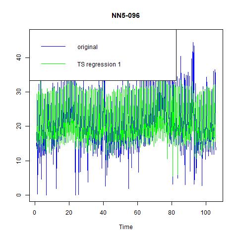

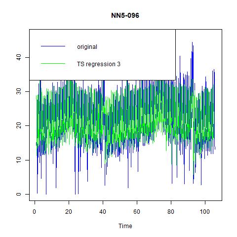
Figure 18 fitted values for three time series regression models for NN5-096
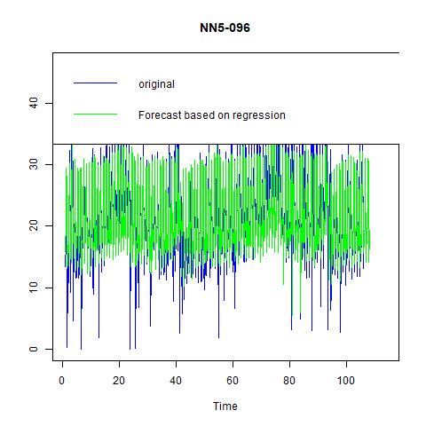
Figure 19 Forecast based on regression with 3 lag and 6 seasonal dummies for NN5-041
3.2.5. Comparison and forecasting Time series forecasting代写
The candidates for best overall model for NN5-096 are ES with ANA, ARIMA (1, 1, 0) with seasonal=7, and time series regression with lags=3 and 6 seasonal dummies. And the last one performs substantially better than the first two, hence we choose it as our final model and forecast 14 values for 2 weeks in figure 19.
4. Conclusion
In this project we apply various estimation and forecasting methods on two times series, namely NN5-041 and NN5-096 to figure out which one performs best in terms of in-sample goodness of fit, measured by indicators such as ME, MSE, and MAPE. These methods include three groups, namely exponential smoothing, ARIMA models, and time series regression and we consider several potential settings for each group. We use the naïve and seasonal naïve method as benchmark, and compare their performance based on the above-mentioned measures. Once we select the best model, we conduct out-of-sample prediction of 14 values for 2 weeks.
The results from our analysis are as follows.
First, for time series NN5-041, we find that: i) exponential smoothing with additive errors, no trends and additive seasonality is best in its class; ii) ARIMA (0, 1, 1) with seasonality = 7 performs better than other ARIMA models; and iii) time series regression with 1 lag and 6 seasonality dummies is the simplest yet informative regression models among our three candidate. And we compare the above three models with the benchmark model of naïve and seasonal naïve models and find that the time series regression model performs the best in terms of less MSE, MAE, and MPAE. So, we choose this one to give out-of-sample forecast for 14 observations.
For NN5-096, we find that: i) exponential smoothing with additive errors, no trends and additive seasonality is best in its class; ii) ARIMA (1, 1, 0) with seasonality = 7 performs better than other ARIMA models; and iii) time series regression with 3 lag and 6 seasonality dummies is the simplest yet informative regression models among our three candidate. And we compare the above three models with the benchmark model of naïve and seasonal naïve models and find that the time series regression model performs the best in terms of less MSE, MAE, and MPAE. So, we choose this one to give out-of-sample forecast for 14 observations.
Appendix: Additive Decomposition for 2 Series
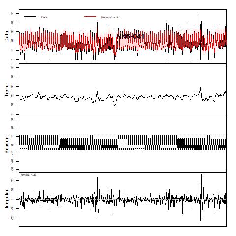
Figure 20 Trend and Season decomposition of NN5-041 (assuming additive decomposition)

Figure 21 Trend and Season decomposition of NN5-096 (assuming additive decomposition)
更多其他: 数学代写 assignment代写 C++代写 代写加急 代码代写 作业代写 作业加急 作业帮助 数据分析代写 编程代写 英国代写 计算机代写
