
Data Science & Machine Learning in Finance (ACCFIN5246)
Individual Assignment – Spring 2023
新西兰商科金融代写 Clearly number each part in your report and structure the answers to follow the same order in Section 4: Q.1, Q.2, Q.3, Q.4 and Q.5.
This assignment counts towards 60% of the overall course grade.
Instruction
— This is an individual assessment.
— Answer all questions listed in Section 4: Q.1, Q.2, Q.3, Q.4 and Q.5.
— Submission to be made electronically via the course Moodle page.
— This submission includes a written report including brief accounts on the logical steps taken,numerical answers, diagrams, and comments (each part in Section 4 specififies how answers are required to be presented).
— Submit only the main report (no additional spreadsheet, nor software routine,etc.).
— Clearly number each part in your report and structure the answers to follow the same order in Section 4: Q.1, Q.2, Q.3, Q.4 and Q.5.
— The project outline presented acorss four sections to develop the implementations, estimation and arrangement of the results.
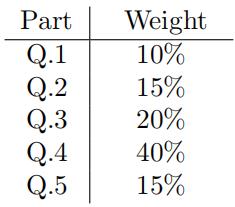
— Each part, within the assignment’s overall grade, carries a weight described below:
— Results should be reported in a clear format. Avoid reporting numbers in the ‘scientifific format’ e.g. 7.2031e-06. All reported numbers should be rounded to two decimal points.
For example, report 0.00 in place of 7.2031e-06.
— The project includes an Appendix (X1) which provides additional data and their descriptions.
— All data, required for the project, is accessible via the course Moodle page.
Section 1: Finance Models 新西兰商科金融代写
Consider the standard and two extended capital asset pricing models characterised below in equa-tions (1)-(3), denoted as Model(A), Model(B) and Model(C), rspectively:
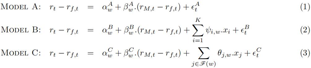
Each model aims at interrelating the real excess equity log-return as the outcome variable, on a given asset rt − rf,t where rf,t is the risk-free log-return, to the right-hand-side explanatory vari-ables, where:
[1.1] Time (daily frequency) is denoted by t = 1, . . . , T and the window index (consecutive days) is denoted by w = 1, . . . , W.
[1.2] Each x-covariate denotes an additional fifinancial, market-level or macroeconomic variable,described in Appendix (X1).
[1.3] x-covariates are indexed by i and j in Model B and Model C, respectively, where i = 1, . . . , K and K describes the number of available covariates in Appendix (X1), whereas j ∈ F(w) refers to a sub-selection of all available covariates. The selected covariates included in set F(w) is carried out based on the learning method described in Section (3). Note that the selection outcome in F(w) is permitted to vary based on the rolling window. 新西兰商科金融代写
[1.4] Specifification error terms are denoted by {![]() } across Models A-C, respectively.
} across Models A-C, respectively.
[1.5] Model constants and CAPM parameters are described by {α![]() } and {
} and {![]() },respectively, in Model A, Model B and Model C. The additional x-covariates are parame-terised according to ψi,w and θj,w, in Model B and Model C, respectively.
},respectively, in Model A, Model B and Model C. The additional x-covariates are parame-terised according to ψi,w and θj,w, in Model B and Model C, respectively.
The object of interest in each model is the time-varying coeffiffifficients described in [1.5]. Each model provides a suggested specifification, ultimately aiming at uncovering the true but unobserved α and β.

Section 2: Data
The focus range covers 2000/01/03-2022/06/03, on a daily basis in Sheet (A) and separately on a monthly basis in Sheet (B). The dataset including all variables are provided on the course Moo-dle page, however you are required to carry out the relevant transformations to convert prices to returns:
[2.1] Observed Amazon Inc. daily stock price (variable AMZN) acquired from the Wharton Research platform (WRDS) is provided towards the construction of (rt) (nominal) log-returns.
[2.2] Observed US daily equity market return (variable SP500) described by the S&P500 composite market index return is provided towards the construction of (rM,t).
[2.3] The nominal daily risk-free log rate (variable rf), associated with the US treasuries is pro-vided such that excess log-returns rt − rf,t and rM,t − rf,t are constructed in real terms.
[2.4] Appendix (X1) provides the description of 14 additional x-covariates (the total variable count is 17 including [2.1], [2.2], [2.3]).
[2.5] All prices in Sheet (A) have to be transformed into returns. All covariances in Sheet (B) to be used without any transformations. 新西兰商科金融代写
[2.6] The eventual dataset including both Sheets (A) and (B) should be in a daily frequency.
To this end, combine both sheets such that monthly frequency data in Sheet (B) are kept constant and repeated identically within each month versus varying other daily observations in Sheet (A).1
[2.7] When there is a missing or non-numeric entry, apply the necessary cleaning. The description sheet provides brief information about the variables. No further information about the variables should be needed, however the variable names are identical to those appearing on WRDS and Fred St. Louis (for the purpose of this assignment you are expected to use the dataset but no further variable research is required).
1For instance, the industrial product index (recorded on ‘2000 01 01’) INDPRO is set equal to the value 91.6261 across all days throughout January 2000.
Section 3: Implementations and Estimation Methodology 新西兰商科金融代写
Implement a code to estimate all three models in equations (1)-(3), on a rolling window basis where w = 25. This indicates that windows include 25 consecutive (working) days as appear in the dataset and rolling forward by one day, amounts to a new window such that each two neighbouring windows overlap for 24 days. For each model, carry out the estimation as described below and store the specifified results for w = 1, . . . , W:
[3.1] To estimate the parameter values described earlier for Model A, use the standard OLS method where only rt − rf,t and rM,t − rf,t are included. The estimation results produce {![]() }.
}.
[3.2] To estimate the parameter values described earlier for Model B, use the standard OLS method where rt − rf,t and rM,t − rf,t are included, in addition to all of the x-covariates included in the Appendix (X1). The estimation results produce {![]() }. 新西兰商科金融代写
}. 新西兰商科金融代写
[3.3] For estimation of the parameter values in Model C, use the Lasso regression method where rt − rf,t and rM,t − rf,t are considered in addition to all of the x-covariates included in the Appendix (X1).The estimation method implements an additional learning parameter λw which determines the selection intensity (λ is characterised as the ‘cost’ associated with the Lasso constraint). Therefore the estimation results associated with the lasso regression produce {![]() }.Once stored the three sets of estimation outpus:
}.Once stored the three sets of estimation outpus: ![]() implement the following secondary regressions:
implement the following secondary regressions:
[3.4] Evaluate the following specififications and store the values for  :
:
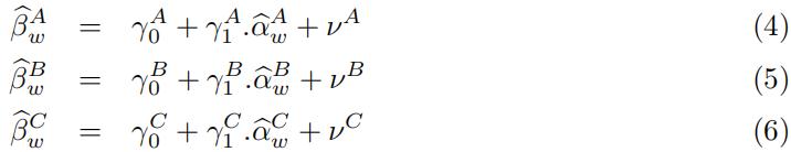
[3.5] Implement a forecasting framework to predict the one-step ahead value of the outcome vari-ables in equations (4)-(6). To carry out the prediction, use 14-consecutive window values earlier obtained: ![]() within each model, to predict the next-step ahead outcome variable value and store the resulting forecast means squared errors (FMSE) values for each of the expressions (4)-(6).
within each model, to predict the next-step ahead outcome variable value and store the resulting forecast means squared errors (FMSE) values for each of the expressions (4)-(6).
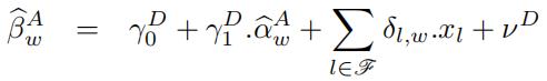
[3.6] Model A uses a minalistic approach without including any x-covariates, whereas Model C applies a learning-based method to select a sub-set of x-covariates. Consider an alternative extended specifification in place of equation (4) based on {![]() } as input data in addition to x-covariates:
} as input data in addition to x-covariates:
 (7)
(7)
where the additional part incorporates the x-covariates,
ν D is the specifification error term, the selection set is determined based on the Lasso approach and l denotes the index for selected x-covariates. This specifification, fifirst, is based on a minimalistic setup of Model A, leading to {![]() } while, second, also informs the secondary regression in (7) through including the additional x-covariates. Note that the estimation is carried out only once and there is no further rolling window implementations in equation (7).
} while, second, also informs the secondary regression in (7) through including the additional x-covariates. Note that the estimation is carried out only once and there is no further rolling window implementations in equation (7).
However, given that {![]() } are already the outcomes of the rolling windows, you will need to set up the new dataset such that each pair
} are already the outcomes of the rolling windows, you will need to set up the new dataset such that each pair ![]() is considered together with the last value of the x-covariates.For instance, window 1 uses the original excess log-returns data from days 1 to 28, inclusive,leading to {
is considered together with the last value of the x-covariates.For instance, window 1 uses the original excess log-returns data from days 1 to 28, inclusive,leading to {![]() }. Then the x-covariate values at day 28 are used to form the second row of dataset required for the estimation of expression (7). Similarly, window 2 uses the original data from days 2 to 29, inclusive, leading to {
}. Then the x-covariate values at day 28 are used to form the second row of dataset required for the estimation of expression (7). Similarly, window 2 uses the original data from days 2 to 29, inclusive, leading to {![]() }. Then the x-covariates at day 29 are used to form the second row of the dataset required for expression (7), etc. This approach ensures that each value for {
}. Then the x-covariates at day 29 are used to form the second row of the dataset required for expression (7), etc. This approach ensures that each value for {![]() } are paired with the most recent values from the x-covariate data, within each window w.
} are paired with the most recent values from the x-covariate data, within each window w.
Section 4: Results and the Final Report 新西兰商科金融代写
Your report should provide the numerical results and comments requested below. Please organise your report following the same structure arranged below by including the answers under parts [Q.1]-[Q.5].
[Q.1] Brieflfly explain the trade-offffs associated between the model variance versus bias-squared to inform model selection. (Concise and less than 200 words) (Mark: 10%)
[Q.2] Report the estimated values for ![]() and their associated p-values. (Mark: 15%) 新西兰商科金融代写
and their associated p-values. (Mark: 15%) 新西兰商科金融代写
[Q.3] Report the FMSE values associated with part [3.5]. Based on these values, provide com-ments which of the expressions (4)-(6) is considered most reliable to predict their outcome variables. (Concise and less than 200 words) (Mark: 20%)
[Q.4] Estimate the specifification expressed in (7) based on the Lasso method. Report the estimated values for {![]() } and their p-values. Explain which of the expressions (6) or (7) is considered more reliable to uncover the underlying relationship between the unobserved true α and β values. Your comments are required to relate your conclusion to the methodologies and estimated values. (Concise and less than 350 words) (Mark: 40%)
} and their p-values. Explain which of the expressions (6) or (7) is considered more reliable to uncover the underlying relationship between the unobserved true α and β values. Your comments are required to relate your conclusion to the methodologies and estimated values. (Concise and less than 350 words) (Mark: 40%)
[Q.5] Construct a diagram for ![]() where the horizontal axis shows w = 1, . . . , W and the vertical axis shows the estimated values obtained for
where the horizontal axis shows w = 1, . . . , W and the vertical axis shows the estimated values obtained for ![]() . Provide brief comments on the interpreta-tion of the depicted cost parameter estimation and why you observe some variations across the windows. Your comments should relate the variations to real economic or fifinancial events during the dataset’s timeline (Concise and less than 200 words). (Mark: 15%)
. Provide brief comments on the interpreta-tion of the depicted cost parameter estimation and why you observe some variations across the windows. Your comments should relate the variations to real economic or fifinancial events during the dataset’s timeline (Concise and less than 200 words). (Mark: 15%)

更多代写:网课代修代修 澳洲pte代考 温哥华会计代考 新加坡edu essay代写 新西兰ArgumentPaper代写 代写大学作业
