微观经济学作业代写 商科作业代写

Microeconomics I

Jehle and Reny (2011) Chapter 1 Consumer Theory

October 1, 2019

微观经济学作业代写 standard properties of utility function u(x) (assumed throughout):• real-valued: u(x) ⊂ R. • continuous: the graph of u(x)

Contents  微观经济学作业代写

1 Primitive Notions                                                                   1

2 Preferences and Utility                                                         1

2.1 Preference Relations . . . . . . . . . . . . . . . . . . . . . . . . . . . . ……………………………. . . 1

2.2 The Utility Function . . . . . . . . . . . . . . . . . . . . . . . . . . . . . ……………………….. . . . . 1

3 The Consumer’s Problem                                                      1

4 Indirect Utility and Expenditure                                         4

4.1 The Indirect Utility Function . . . . . . . . . . . . . . . . . . . . . …………. . . . . . . . . . . . . . 4

4.2 The Expenditure Function . . . . . . . . . . . . . . . . . . . . . . . . . ……….. . . . . . . . . . . . . 6

4.3 Relations Between the Two . . . . . . . . . . . . . . . . . . . . . . . . . ………….. . . . . . . . . . . 9

5 Properties of Consumer Demand                                       10 微观经济学作业代写

5.1 Relative Prices and Real Income . . . . . . . . . . . . . . . . . . . . ………. . . . . . . . . . . . . 10

5.2 Income and Substitution Effffects . . . . . . . . . . . . . . . . . . . . . …. . . . . . . . . . . . . . 11

5.3 Some Elasticity Relations . . . . . . . . . . . . . . . . . . . . . . ………… . . . . . . . . . . . . . . . 13

1 PrimitiveNotions

2 Preferences andUtility

2.1 PreferenceRelations

2.2 The UtilityFunction

3 TheConsumer’s  Problem

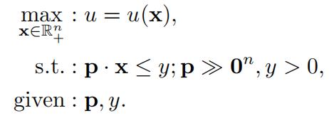
the consumer’s utility maximization problem:

---

∗E-mail: <tnaito@waseda.jp>; homepage: <http://www.f.waseda.jp/tnaito>.

• x= (x₁, …, x_i, …, x_n)^T : consumption vector (consumption bundle)
• u:utility
• p= (p₁, …, p_i, …, p_n)^T : price vector
• y:income

budget constraint p · x ≤ y: total expenditure must be no greater than income 微观经济学作业代写

• budget set: the set of x such that the budget constraintholds
• budget line: the set of x such that the budget constraint holds withequality

JR Figure 1.9:

• y/p_i: real income in terms of good i: how many units of good i one can buy withy

(i-intercept of the budget line)微观经济学作业代写

• p_i/p_j: relative price of good i to good j (price of good i in terms of good j) (absolutevalue of the slope of the budget line from the i-axis):

-how many units of good j one can buy by giving up one unit of goodi

-howmany units of good j one must give up to buy one unit of good i (market value)

standard properties of utility function u(x) (assumed throughout):

• real-valued: u(x) ⊂R.
• continuous: the graph of u(x) does not have any jumpingpart
• strictly increasing: u(x¹) > u(x⁰) for x¹≫ x⁰.

(⇐ u_i(x) > 0∀i: marginal utility of good i is positive)

• strictlyquasiconcave:  u((1 − t)x¹ + tx²) > min[u(x¹), u(x²)]∀x¹, x², x² ƒ= x¹∀t ∈ (0, 1).

JR Figure 1.8:

• indifferencecurve ∼ (x⁰) ≡ {x|x ∈ Rⁿ , u(x) = u(x⁰)}:  the set of x giving the same utility as x⁰
• u(x) is strictly increasing ⇒ each indifference curve isdownward-sloping
• u(x) is strictly quasiconcave ⇒ each indifference curve is strictly convex to theorigin
• MRS_ij(x) ≡ −dx_j/dx_i|_du=0 = u_i(x)/u_j(x):  marginal rate of substitution of good i for good j¹

(absolute value of the slope of an indifference curve from the i-axis):  微观经济学作业代写

-how many units of good j one is willing to get by giving up one unit of goodi

–how many units of good jone is willing to give up to get one unit of good i (subjective value)

---

1 There is confusion about how to call M RS_ij (x) ≡ −dx_j /dx_i|_du=0 the marginal rate of substitution of which good for whichother good.  JR (p.  12) calls:  “the rate at which the consumer is just willing to give up good two per unit of good one received”“the  marginal  rate  of  substitution  of  good  two  for  good  one”.   However,  several  English  language  dictionaries  say  that  “yousubstitute A for B” means “you decrease B and increase A”.  If we follow the dictionary definition, JR should have called that“the marginal rate of substitution of good one for good two” just like us.微观经济学作业代写

Anyway, the important thing is not to argue which good comes first, but to understand the authors’ definition every time.

• u(x) is strictly quasiconcave ⇒ diminishing marginal rate ofsubstitution

JR Figure 1.10:

necessary conditions for the solution x^∗:

• budgetbalancedness: p  x^∗ = y (what if p · x^∗ < y?)
• indifference curve is tangent to budget line: M RS_ij(x^∗) = p_i/p_j(what if M RS_ij(x^∗) ≷ p_i/p_j?)

JR Figure 1.11:

• Marshallian (ordinary) demand function x^∗= x(p, y)
• (a):p¹ < p⁰ → x₁(p¹, p⁰, y⁰) > x₁(p⁰, p⁰, y⁰) usually
• (b): Marshallian (ordinary) demand curve is usually downward-sloping in the (x₁, p₁)-plane Lagrangian method (see section 7.2, MathApps): 微观经济学作业代写

p · x ≤ y

y − p · x ≥ 0

L(x, λ) ≡ u(x) + λ(y − p · x).

u(x) is strictly increasing ⇒ y − p · x = 0 (budget balancedness):

L_i(x, λ) = u_i(x) − λp_i = 0, i = 1, …, n, (1)

L_λ(x, λ) = y − p · x = 0. (2)

(1):

u_i(x)/u_j(x) = p_i/p_j, i, j = 1, …, n. (3)

• (2), (3) are the same as the two necessary conditions in JR Figure10
• u(x)is strictly quasiconcave, g(x) ≡ p  x is linear (⇒ quasiconvex) ⇒ (1), (2) are sufficient (see section 7.4, Math Apps)

Example 1 (see JR Example 1.1)

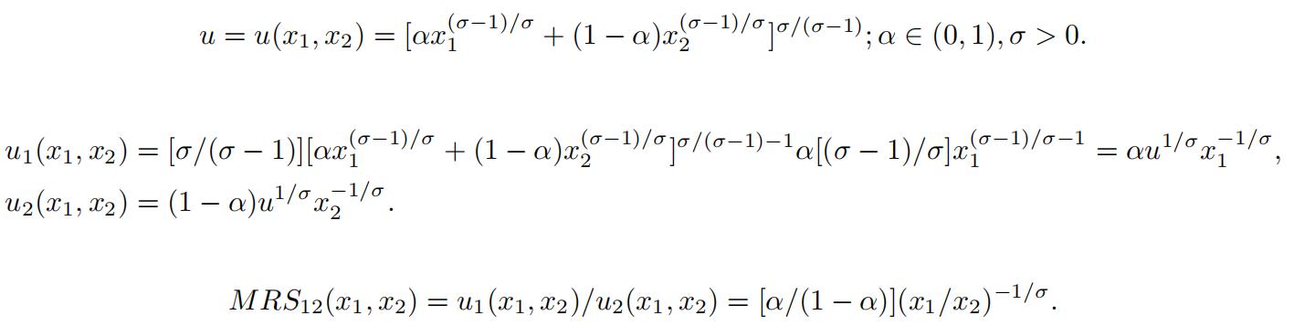
CES (constant elasticity of substitution) utility function:

(3):

[α/(1 − α)](x₁/x₂)^−1/σ = p₁/p₂. (4)

elasticity of substitution between goods 1 and 2:

ES₁₂(x₁, x₂) ≡ −∂ ln(x₁/x₂)/∂ ln(p₁/p₂).

(4):

ln[α/(1 − α)] − (1/σ) ln(x₁/x₂) = ln(p₁/p₂)

−(1/σ)d ln(x₁/x₂) = d ln(p₁/p₂)

d ln(x₁/x₂)/d ln(p₁/p₂) = −σ.

ES₁₂(x₁, x₂) = σ.

(2), (4):

x₁(p₁, p₂, y) = (p₁/α)^−σP (p₁, p₂)^σ−1y, (5)

x₂(p₁, p₂, y) = [p₂/(1 − α)]^−σP (p₁, p₂)^σ−1y; (6)

P (p₁, p₂) ≡ {α(p₁/α)^1−σ + (1 − α)[p₂/(1 − α)]^1−σ }^1/(1−σ). (7)

special cases:

• σ =0 : u(x₁, x₂) = min[x₁, x₂]: Leontief
• σ= 1 : u(x₁, x₂) = x^αx^1−α:  Cobb–Douglas
• σ =∞ : u(x₁, x₂) = αx₁ + (1 − α)x₂: linear

in Leontief or linear case, (1) (and hence (3), (4)) does not apply automatically

4 Indirect Utility and Expenditure

4.1 The Indirect Utility Function

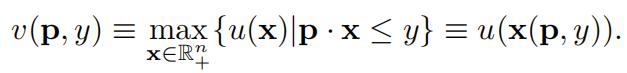
the consumer’s indirect utility function:

JR Figure 1.13:

• v(p, y) corresponds to the indifference curve at the solution x^∗= x(p, y)

Theorem 1 (Properties of the Indirect Utility Function) v(p, y) is:

1. continuous;
2. homogeneous of degree zero in (p,y);
3. strictly increasing iny;
4. decreasing inp;
5. quasiconvex in (p,y);
6. satisfiesRoy’s  identity:

x_i(p, y) = −(∂v(p, y)/∂p_i)/(∂v(p, y)/∂y), i = 1, …, n.

Note that only property 6 requires differentiability.

Proof. See proof of JR Theorem 1.6.

alternative proof of properties 5 and 6:

5:

For (p¹, y¹) and (p², y²), let p^t ≡ (1 − t)p¹ + tp², y^t ≡ (1 − t)y¹ + ty²; t ∈ [0, 1]. For (p^t, y^t), the budget constraint implies:

p^t · x ≤ y^t

[(1 − t)p¹ + tp²] · x ≤ (1 − t)y¹ + ty²

(1 − t)p¹ · x + tp² · x ≤ (1 − t)y¹ + ty²

⇒ p¹ · x ≤ y¹ or p² · x ≤ y².

 

p¹ · x ≤ y¹ ⇒ v(p^t, y^t) ≤ v(p¹, y¹),

p² · x ≤ y² ⇒ v(p^t, y^t) ≤ v(p², y²).

∴ v(p^t, y^t) ≤ max[v(p¹, y¹), v(p², y²)].

6:

Differentiating v(p, y) ≡ u(x(p, y)) with respect to y gives:

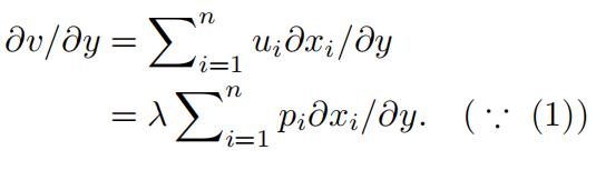
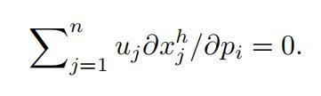
Differentiating p · x(p, y) ≡ y with respect to y gives:

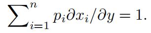
This implies that:

Differentiating v(p, y) ≡ u(x(p, y)) with respect to p_i gives:

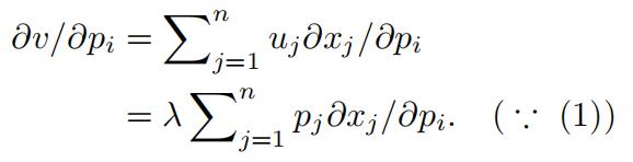
Differentiating p · x(p, y) ≡ y with respect to p_i gives:

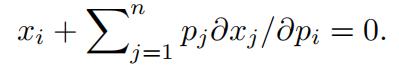
This implies that:

∂v/∂p_i = −λx_i.

Therefore, we obtain:

x_i = −(∂v/∂p_i)/(∂v/∂y).

note:

• economic meaning of λ: the value of relaxing (or tightening) theconstraint

Example 2 (see JR Example 1.2)

(5), (6):

v(p₁, p₂, y) = y/P (p₁, p₂). (8)

(8):

∂v(p₁, p₂, y)/∂y = 1/P > 0,

∂v(p₁, p₂, y)/∂p₁ = −(y/P ²)∂P/∂p₁

= −(y/P ²)[1/(1 − σ)]{·}^{1/(1−σ)−1}α(1 − σ)(p₁/α)^1−σ−1(1/α)

= −(y/P ²)P ^σ(p₁/α)^−σ < 0,

∂v(p₁, p₂, y)/∂p₂ = −(y/P ²)P ^σ[p₂/(1 − α)]^−σ < 0.

 

− (∂v(p₁, p₂, y)/∂p₁)/(∂v(p₁, p₂, y)/∂y)

= [(y/P ²)P ^σ(p₁/α)^−σ]/(1/P )

= (y/P )P ^σ(p₁/α)^−σ = x₁(p₁, p₂, y),

− (∂v(p₁, p₂, y)/∂p₂)/(∂v(p₁, p₂, y)/∂y)

= {(y/P ²)P ^σ[p₂/(1 − α)]^−σ}/(1/P )

= (y/P )P ^σ[p₂/(1 − α)]^−σ = x₂(p₁, p₂, y).

4.2 The Expenditure Function

the consumer’s expenditure minimization problem:

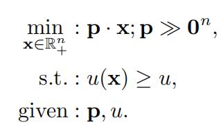
JR Figure 1.15:

necessary conditions for the solution x^∗:

• minimumutility constraint is satisfied with equality: u(x) = u (what if u(x) > u?)
• iso-expenditure line is tangent to indifference curve: p_i/p_j= M RS_ij(x^∗) (what if p_i/p_j ≷ M RS_ij(x^∗)?)

JR Figure 16:

• Hicksian (compensated) demand function x^∗= x^h(p, u)
• (a):p¹ < p⁰ → x^h(p¹, p⁰, u) > x^h(p⁰, p⁰, u)
• (b): Hicksian (compensated) demand curve is downward-sloping in the (x₁, p₁)-plane Lagrangian method (see section 7.2, MathApps):

u(x) ≥ u u − u(x) ≤ 0

L(x, λ) ≡ p · x + λ(u − u(x)).

p · x is strictly increasing ⇒ u − u(x) ≤ 0 is satisfied with equality:

L_i(x, λ) = p_i − λu_i(x) = 0, i = 1, …, n, (9)

L_λ(x, λ) = u − u(x) = 0. (10)

(9):

p_i/p_j = u_i(x)/u_j(x), i, j = 1, …, n. (11)

• (10), (11) are the same as the two necessary conditions in JR Figure15
• f(x) ≡ p  x is linear (⇒ quasiconvex), u(x) is strictly quasiconcave ⇒ (9), (10) are sufficient (see section 7.4, Math Apps)

the consumer’s expenditure function:

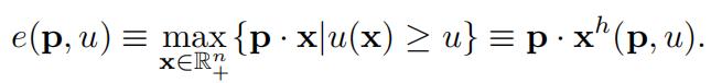
JR Figure 1.15:

• e(p,u) corresponds to the iso-expenditure line at the solution x^∗ = x^h(p, u)

Theorem 2 (Properties of the  Expenditure Function)  e(p, u) is:  1. e(p, u(0ⁿ)) = 0; 微观经济学作业代写

1. e(p, u(0n)) = 0;
2. continuous;
3. strictly increasing in u;
4. increasing in p;
5. homogeneous of degree one in p;
6. concave in p;
7. satisfifies Shephard’s lemma:

∂e(p, u)/∂p_i = x^h(p, u), i = 1, …, n.

Note that only property 7 requires differentiability.

Proof. See proof of JR Theorem 1.7.

alternative proof of properties 6 and 7:

6:

With u given, let x¹ and x² be the solution to p¹ and p², respectively. Also, let p^t ≡ (1 − t)p¹ + tp², t ∈[0, 1], and let x^t be the solution to p^t. Then we have:

p¹ · x¹ ≤ p¹ · x^t,

p² · x² ≤ p² · x^t.

Multiplying the first and second inequalities by (1 − t) and t, respectively, and summing them up, we obtain:

(1 − t)p¹ · x¹ + tp² · x² ≤ (1 − t)p¹ · x^t + tp² · x^t = p^t · x^t.

∴ (1 − t)e(p¹, u) + te(p², u) ≤ e(p^t, u).

7:

Differentiating e(p, u) ≡ p · x^h(p, u) with respect to u gives:

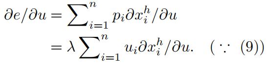
Differentiating u(x^h(p, u)) ≡ u with respect to u gives:

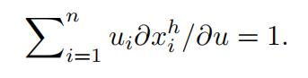
This implies that:

∂e/∂u = λ.

Differentiating e(p, u) ≡ p · x^h(p, u) with respect to p_i gives:  微观经济学作业代写

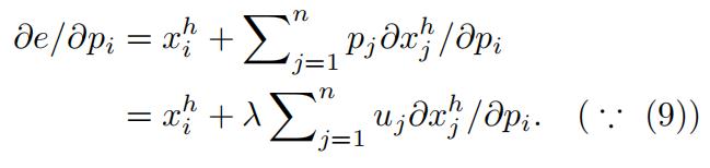
Differentiating u(x^h(p, u)) ≡ u with respect to p_i gives:

This implies that:

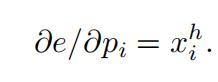
notes:

• economic meaning of λ: the value of relaxing (or tightening) theconstraint
• economic meaning of concavity of e(p, u) in p:

even if p_i increases, e increases less than linearly (∵ x^h adjusts to minimize e)

Example 3 (see JR Example 1.3)

u = u(x  , x  ) = [αx^(σ−1)/σ + (1 − α)x^(σ−1)/σ ]^σ/(σ−1); α ∈ (0, 1), σ > 0.

(11):

p1/p2 = [α/(1 − α)](x1/x2)−1/σ .(see (4)) (12)

(10), (12):

p₁/p₂ = [α/(1 − α)](x₁/x₂)^−1/σ.    (see (4)) (12)  微观经济学作业代写

x^h(p₁, p₂, u) = (p₁/α)^−σP (p₁, p₂)^σu, (13)

x^h(p₁, p₂, u) = [p₂/(1 − α)]^−σ P (p₁, p₂)^σu; (14)

(13), (14):

P (p₁, p₂) = {α(p₁/α)^1−σ + (1 − α)[p₂/(1 − α)]^1−σ}^1/(1−σ).    (see (7))

e(p₁, p₂, u) = P (p₁, p₂)u. (15)

(15):

∂e(p₁, p₂, u)/∂p₁ = (∂P/∂p₁)u

= [1/(1 − σ)]{·}^{1/(1−σ)−1}α(1 − σ)(p₁/α)^1−σ−1(1/α)u  微观经济学作业代写

= P ^σ(p₁/α)^−σu = x^h(p₁, p₂, u),

∂e(p₁, p₂, u)/∂p₁ = (∂P/∂p₂)u

= P ^σ[p₂/(1 − α)]^−σu = x^h(p₁, p₂, u).

4.3 Relations Between the Two

JR Figure 1.18 (a):

• for(p, y), the utility-max solution is x^∗ = x(p, y), which gives v(p, y)

→ for (p, v(p, y)), the expenditure-min solution is x^∗ = x^h(p, v(p, y)), which gives e(p, v(p, y)) = y

• for (p, u), the expenditure-min solution is x^∗= x^h(p, u), which gives e(p, u) 微观经济学作业代写

→ for (p, e(p, u)), the utility-max solution is x^∗ = x(p, e(p, u)), which gives v(p, e(p, u)) = u

Theorem 3 (Relations between Indirect Utility and Expenditure Functions) .

1. y ≡ e(p, v(p,y)).
2. u ≡ v(p, e(p,u)).

Theorem 4 (Relations between Marshallian and Hicksian Demand Functions) .

1.  x(p, y) ≡x^h(p, v(p, y)).
2. x^h(p, u) ≡ x(p, e(p, u)).

Example 4 (see JR Examples 1.4, 1.5)

(8), (15):

v(p₁, p₂, y) = y/P (p₁, p₂),

e(p₁, p₂, u) = P (p₁, p₂)u.  微观经济学作业代写

verify Theorem 3:

e(p₁, p₂, v(p₁, p₂, y)) = P (p₁, p₂)y/P (p₁, p₂) = y,

v(p₁, p₂, e(p₁, p₂, u)) = P (p₁, p₂)u/P (p₁, p₂) = u.

use Theorem 3, 1. to derive v(p, y) from e(p, u):

y = e(p₁, p₂, v(p₁, p₂, y)) = P (p₁, p₂)v(p₁, p₂, y)

⇒ v(p₁, p₂, y) = y/P (p₁, p₂).  微观经济学作业代写

use Theorem 3, 2. to derive e(p, u) from v(p, y):

u = v(p₁, p₂, e(p₁, p₂, u)) = e(p₁, p₂, u)/P (p₁, p₂)

⇒ e(p₁, p₂, u) = P (p₁, p₂)u.

∴ once we obtain either v(p, y) or e(p, u), we can derive the other from Theorem 3 (5), (6), (13), (14):

verify Theorem 4:

x₁(p₁, p₂, y) = (p₁/α)^−σP (p₁, p₂)^σ−1y,

x₂(p₁, p₂, y) = [p₂/(1 − α)]^−σP (p₁, p₂)^σ−1y,

x^h(p₁, p₂, u) = (p₁/α)^−σP (p₁, p₂)^σu,

x^h(p₁, p₂, u) = [p₂/(1 − α)]^−σP (p₁, p₂)^σu. 微观经济学作业代写

 

x^h(p₁, p₂, v(p₁, p₂, y)) = (p₁/α)^−σP (p₁, p₂)^σy/P (p₁, p₂) = x₁(p₁, p₂, y),

x^h(p₁, p₂, v(p₁, p₂, y)) = [p₂/(1 − α)]^−σ P (p₁, p₂)^σy/P (p₁, p₂) = x₂(p₁, p₂, y),

x₁(p₁, p₂, e(p₁, p₂, u)) = (p₁/α)^−σP (p₁, p₂)^σ−1P (p₁, p₂)u = x^h(p₁, p₂, u),

x₂(p₁, p₂, e(p₁, p₂, u)) = [p₂/(1 − α)]^−σ P (p₁, p₂)^σ−1P (p₁, p₂)u = x^h(p₁, p₂, u).

5 Properties of Consumer Demand 微观经济学作业代写

5.1 Relative Prices and Real Income

Theorem 5 (Homogeneity and Budget Balancedness) The Marshallian demand function x(p, y):

1. ishomogeneous of degree zero:  x(tp, ty) = x(p, y)∀t > 0;
2. satisfies budget balancedness: p x(p, y) =y.

Proof. For  property 1., the budget constraint for (tp, ty) is tp · x ≤ ty. Dividing both sides by t > 0 gives p · x ≤ y, which is equivalent to the budget constraint for (p, y). This implies that x(tp, ty) = x(p, y). Property 2. immediately follows from strict increasingness of u(x).

implication of Theorem 5, 1.:  微观经济学作业代写

let the last good n be the numeraire (unit of measurement):

t = 1/p_n : x(p, y) = x(p₁/p_n, …, p_n−1/p_n, 1, y/p_n).

we can effectively reduce the dimension of independent variables by one

5.2 Income and Substitution Effects

income effect on demand for good 1:

• y ↑ → x₁↑: good 1 is a normal good
• y ↑ → x₁unchanged: good 1 is a neutral good
• y ↑ → x₁↓: good 1 is an inferior good (e.g., staple foods such as potato, noodles, rice, )

JR Figure 1.19:  微观经济学作业代写

own price effect on demand for good 1:

• (a): p₁↓ → x₁ ↑: good 1 is an ordinary good
• (b): p₁↓ → x₁ unchanged
• (c): p₁↓ → x₁ ↓: good 1 is a Giffen good (e.g.,  staple foods  such as potato, noodles,  rice, etc.) Q: what determines if a good is ordinary or Giffen?

two effects that are common to (a)–(c) of JR Figure 1.19:

• p₁/p₂= M RS₁₂ ↓
• u ↑ (just as income↑)

idea: neutralize the second effect to extract only the first effect JR Figure 1.20 (a):

• p¹< p⁰ → x¹ > x⁰, u¹ > u⁰
• hypothetically reduce income so that the consumer is left withu⁰

→ find the tangent point x^s between the old indifference curve u⁰ and the hypothetical budget line

x⁰ → x^s: substitution effect: caused by the change in p, with u given (i.e., Hicksian demand change)  微观经济学作业代写

• hypothetically turn income back → u⁰increases to u¹

x^s → x¹: income effect: caused by the change in u (i.e., income), with p given

JR Figure 1.20 (b):

• p¹< p⁰ → x¹ > x⁰ along the Marshallian demand curve (see JR Figure 1.11 (b))
• p¹< p⁰ → x^s > x⁰ along the Hicksian demand curve (see JR Figure 1.16 (b))
• the difference between the Marshallian and Hicksian demand curves is the incomeeffect

Theorem 6 (The Slutsky Equation) .

where u = v(p, y).

Proof. Differentiating x^h(p, u) ≡ x_i(p, e(p, u)) from Theorem 4, 2. with respect to p_j gives:

∂x^h(p, u)/∂p_j = ∂x_i(p, e(p, u))/∂p_j + (∂x_i(p, e(p, u))/∂y)∂e(p, u)/∂p_j

= ∂x_i(p, e(p, u))/∂p_j + (∂x_i(p, e(p, u))/∂y)x^h(p, u). ( ∵ Theorem 2, 7.) 微观经济学作业代写

Using y ≡ e(p, v(p, y)) from Theorems 3, 1., x^h(p, u) ≡ x_i(p, e(p, u)) from Theorem 4, 2., and u = v(p, y),

this is rewritten as:

∂x^h(p, u)/∂p_j = ∂x_i(p, y)/∂p_j + (∂x_i(p, y)/∂y)x_j(p, y).

Moving the second term of the right-hand side to the other side, we obtain the desired result.

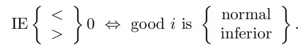
signs of SE and IE for the own price effect (j = i):

Theorem 7 (Negative Semideftnite Substitution Matrix) The substitution matrix:

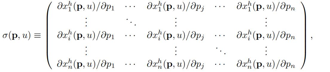
is symmetric and negative semidefinite:

z^T σ(p, u)z ≤ 0∀z ∈ Rⁿ.

Proof. Since the (i, j)th element  of σ(p, u)  is ∂x^h(p, u)/∂p_j  =  ∂²e(p, u)/(∂p_j∂p_i) from Theorem 2,  7., σ(p, u) is the Hessian matrix of e(p, u) with respect to p. Since e(p, u) is concave in p from Theorem 2, 6., its Hessian matrix σ(p, u) is negative semidefinite from Theorem 15, Math Apps. Symmetry follows from Theorem 13, Math Apps (Young’s Theorem).

Theorem 8 (Negative Own-Substitution Terms) The own substitution effect is nonpositive: 微观经济学作业代写

∂x^h(p, u)/∂p_i ≤ 0, i = 1, …, n.

Proof.  Applying z = (0, …, z_i, …, 0)^T ; z_i  =ƒ 0 to Theorem 7 gives (∂x^h(p, u)/∂p_j)z² ≤ 0. Since z² > 0, we obtain ∂x^h(p, u)/∂p_j ≤ 0.

JR Figure 1.19:

own price effect on demand for good 1:

• (a): good 1 is normal → SE < 0, IE < 0 → good 1 isordinary
• (b):good 1 is inferior → SE < 0, IE > 0 → good 1 is neither ordinary nor Giffen
• (c): good 1 is inferior → SE < 0, IE > 0 → good 1 isGiffen

Theorem 9 (The Law of Demand) . 

1. If a good is a normal good, then the good is an ordinary
2. If a good is a Giffen good, then the good is an inferior

5.3 Some Elasticity Relations 微观经济学作业代写

Deftnition 1 (Demand Elasticities and Income Shares) .

• income elasticity of demand for good i: η_i≡ ∂ ln x_i(p, y)/∂ ln y;
• cross-price elasticity of demand for good i with respect to p_j: ε_ij≡ ∂ ln x_i(p, y)/∂ ln p_j; (own-price elasticity of demand for good i if j = i)
• income share (or “expenditure share”) of good i: s_i≡ p_ix_i(p, y)/y; s_i ≥ 0, Σns_i = 1.

Theorem 10 (Aggregation in Consumer Demand) .

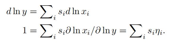
1. Engelaggregation: Σn s_iη_i = 1;
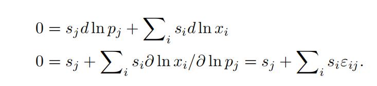
2. Cournotaggregation: Σn s_iε_ij = −s_j.

Proof. Logarithmically differentiating y = Σn

p_ix_i gives:

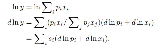
First, let d ln y ƒ= 0, d ln p_i = 0∀i. Then we have:

Second, let d ln p_j =ƒ 0, d ln y = d ln p_i = 0∀i j. Then we have:

其他代写：代写CS C++代写 java代写 matlab代写 web代写 app代写 作业加急 物理代写 数学代写 考试助攻 paper代写 r代写 金融经济统计代写 finance代写

合作平台：essay代写 论文代写 写手招聘 英国留学生代写