
Q1
differences estimator代写 A classic application of difference-in-differences estimator is the study of the effect of job training program
A classic application of difference-in-differences estimator is the study of the effect of job training program on earnings. Suppose now we want to study if participating a job training program enable workers to earn more. We have a panel data on the earnings of workers before and after a certain period when a job training program is available. Our data also records whether each of the workers participate in the job training program. To estimate the effect of participating a job training program on workers’ earnings, simply comparing the earnings of participants (“treated”) and non-participants (“untreated”) will not be convincing.
Intuitively,differences estimator代写
the simple “differences estimator” ignores unobserved differences between the treated and untreated individuals, and the differences can be correlated with their earnings. So, the simple “differences estimator” can be biased. For example, those who participate in job training program may be more motivated to work anyways, so would earn more than non-participants even without training program. In this case, the “differences estimator” overestimates the effect of the program. Another potential estimation of the effect of participating a job training program on workers’ earnings is by comparing the earnings of individuals who participate before and after “treatment” (in panel data set). However, this can also be biased since there may be a time trend for the earnings.
To better analyze this problem, we can use difference-in-differences estimator. Intuitively, we difference out time-constant (level) differences between treatment and control and time-trends to isolate the effect of the effect of job training program. In detail, let A be the control(untreated) group and B the treatment group. The model can be summarized as
![]()
Where y is the earnings of the workers, dB captures possible differences between the treatment and control groups prior to the policy change. d2 captures aggregate factors that would cause changes in y over time even in the absence of a policy change. The coefficient of interest is . The difference-in-differences (DD) estimator is
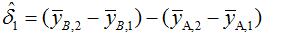
With difference-in-differences (DD) estimate method, the time-constant (level) differences between treatment and control and time-trends are differenced out, we can get a better estimation of the effect of job training program.
Q2
a)
To implement the two-stage least squares estimation, we first regress on w1, z , z and (k=1,2…K). That is, to estimate (first stage of estimation)
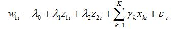
Then, substitute the fitted value of , which is , into the estimation equation (the second stage of estimation)
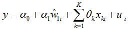
Then, we can get the two-stage least squares estimator of
b)
For two-stage least squares estimator in a) to be satisfactory (for z , z to be appropriate instrument variables (IVs)), we need to assume that and , i.e.z, z, are not correlated with . Also, we need to assume z , z are partially correlated with w , i.e., in the first stage of estimation

We need . (In fact, we may just need one instrument variable in this problem, so, it may differences estimator代写
be okay to have one of , to satisfy the corresponding properties.)
c)
We can test whether z , z are partially correlated with w, but cannot test if z ,
z are not correlated with u. To test if z , z are partially correlated with , the null is
that this condition fails: . In the estimation

we can use the heteroskedasticity-robust joint F statistic on z , z (that is, for ). If
the p-value is suitable small (certainly under 0.05), we might not reject that z , z are
partially correlated with .
We cannot directly test if , are not correlated with since is not directly
observable.
Q3 differences estimator代写
a)
From the setting of the model, we have![]()

So
Thus, we have
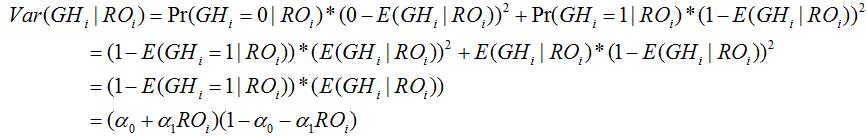
Therefore
depends on RO, so we must account for heteroskedasticity with this linear probability model.
b)
If , the OLS estimator of the linear probability model can be inconsistent. This can be seen from the below equation.differences estimator代写
![]()
In fact, we may need a stronger assumption that ![]() to make our analysis more convenient. But given the fact that individuals are randomly offered subsidized health insurance, it is plausible that we assume cov
to make our analysis more convenient. But given the fact that individuals are randomly offered subsidized health insurance, it is plausible that we assume cov ![]() hold.
hold.
Besides, as we can see from a), heteroskedasticity presents in the model, so for the estimator to be efficient, we need to correct for the heteroskedasticity (for example, use robust standard errors).
Another important fact is when estimated GH is beyond 0 to 1, the OLS estimator will no longer be consistent, this is one of the weak points of linear probability model.
c)
It will not be possible for a model to take all the characteristics in analysis. In our model, we focus only on the relationship between good health and want to get a good estimator of the coefficient a. The omitted variable bias happens when the omitted variable is correlated with RO, which makes cov ![]() . But from b), this is not likely to happen.
. But from b), this is not likely to happen.
Q4
a)
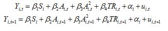
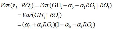
From the setting of the model, we have
for t=1,2. Thus
![]()
Where ![]() , note that is rewrite as to avoid confusing.
, note that is rewrite as to avoid confusing.
To estimate the causal effect of training on income (β), we use ordinary least square(OLS) method on the difference equations to get β. For OLS to be a satisfactory method, we need △TR,△u to not be correlated. Note that TR=0, ![]() are not correlated, we also need
are not correlated, we also need ![]() are not correlated. With the differenced equation, we cannot estimate the coefficient on S since S, which represents a time invariant effect, is eliminated from the differencing process.
are not correlated. With the differenced equation, we cannot estimate the coefficient on S since S, which represents a time invariant effect, is eliminated from the differencing process.
b)
Since UR is likely to be correlated with TR, u and is not correlated with u ,u we can
use it as an instrument variable in estimating the difference equation. We can first run the first stage regression
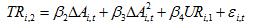
and substitute the fitted value of TR(TR) into the second stage of the estimation
![]()
Where ![]() . The estimated β is a satisfactory estimator for the effect of training.
. The estimated β is a satisfactory estimator for the effect of training.

更多其他: 数学代写 assignment代写 数据分析代写 程序代写 算法代写 经济代写 代写CS C++代写 编程代写 英国代写
