Main Report
analysis techniques代写 This project demonstrates the time series analysis techniques for analyzing two time series data.

Introduction
This project demonstrates the time series analysis techniques for analyzing two time series data. The popular and classical autoregressive moving-average (ARMA) model, generalized autoregressive conditional heteroskedasticity (GARCH) model, and vector autoregression (VAR) model are applied on the adjusted close price of the JMP Group LLC (JMP.N) and International Business Machines Corporation (IBM.N) from 2015-01-02 to 2018-12-04.analysis techniques代写
JMP.N is a company listed in NYSE with full-service in investment banking and asset management. While IMB.N is a technology company listed in NYSE also with services in cognitive solutions, global business, technology & cloud platforms, systems and global Financing.
It is believed that the stick prices of above two companies have their own dynamic pattern but also high relative because of the high correlation of the big firms in the US or global economy.
To study their own dynamics of the corresponding stock price, ARMA and GARCH models are employed for individual analysis. Further, the two time series data sets are combined together and investigated jointly through a VAR model.analysis techniques代写
It is well-known that the price itself is non-stationary.
The most common way to deal with such non-stationary stock price data in practice is to take the logarithm of the price difference. Thus, the numerical value, which still attains interpretability, represents the percentage daily return of the stock. After such practice, the transformed time series is very likely to be stationary, the case where further advanced time series techniques could be applied.
ARMA modeling
The initial step one shall starts with is to fit a stationary model. A stationary ARMA(p,q) models implies that the null hypothesis that the time series has no trend is not able to be rejected.analysis techniques代写
-
Case 1: JPM.N
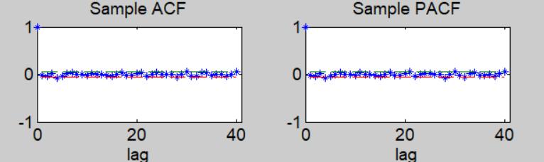
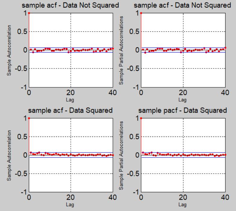
For the first JMP.N data, one are able to calculate the ACF and PACF of the log return series, the left panel of the figure below shows the corresponding ACF while the right panel shows the corresponding. It is easy to see that the series is stationary at time lag 1, indicating that the null hypothesis that the time series has no trend after time lag 1 is not able to be rejected. Thus, one are able pick the initial choice of parameter for AR(p) p=1, and for MA(q) q=1;
Through the ACF and PACF suggest a ARMA(1,1) model, the model seems to be too trivial to has a good performance in forecasting due to the lacks of information.
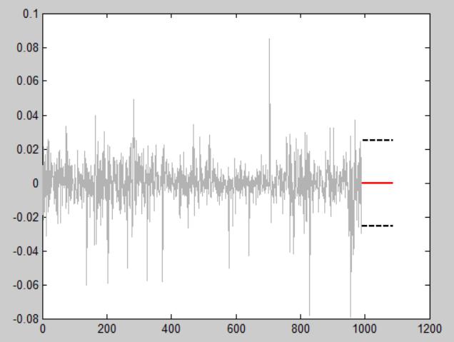
The Figure below indeed demonstrates the failure of forecasting through a ARMA(1,1) model.analysis techniques代写
Forecast the following 100 periods, the predicted values have no variability.
The reason might be the that the assumption of ARMA model, the error terms is a while noise process, is violated in this real data case. The model takes the heteroskedasticity into consideration is suggested.
-
Case 2: IBM.N
The procedure of ARMA modelling for the IBM.N is similar to that of the JPM.N data. According to the ACF and PACF plot below, the result is very similar to that of the ARMA model of JMP.N.
An ARMA(1,1) model is selected. Nevertheless, the predictability of such an ARMA(1,1) is unsatisfactory still. analysis techniques代写
Forecast the following 100 periods, the predicted values have no variability.
The reason might be the that the assumption of ARMA model, the error terms is a while noise process, is violated in this real data case. The model takes the heteroskedasticity into consideration is suggested.analysis techniques代写
GARCH modeling
Based on the failure of the ARMA model above, a more advanced GARCH model is applied for these two times series data, respectively.
-
Case 1: JPM.N
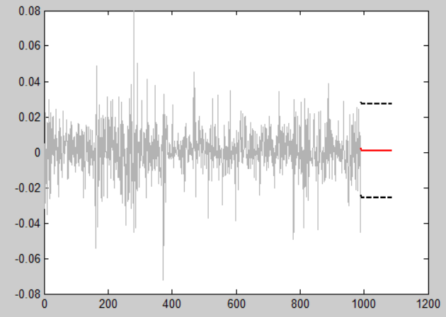
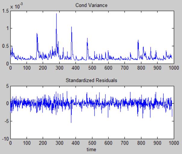
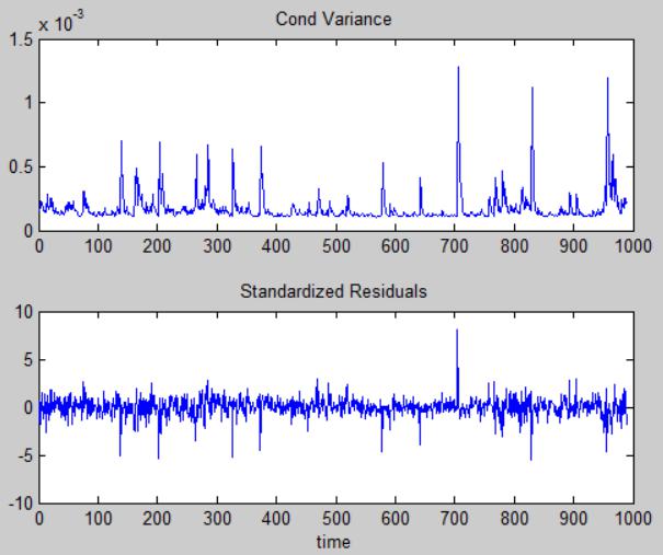
Conditional variance and standardized residuals of GARCH(1,1) are plotted as followings. It is easy to see that the conditional variance of the residuals, or more particularity, the conditional validity has a high persistency. That is, the momentums of the conditional variance are able to keep several days. The bottom panel of the below figure shows the standard residuals. The standard residual is very likely to be a white noise process.analysis techniques代写
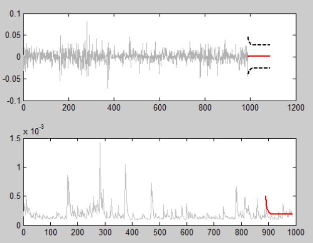
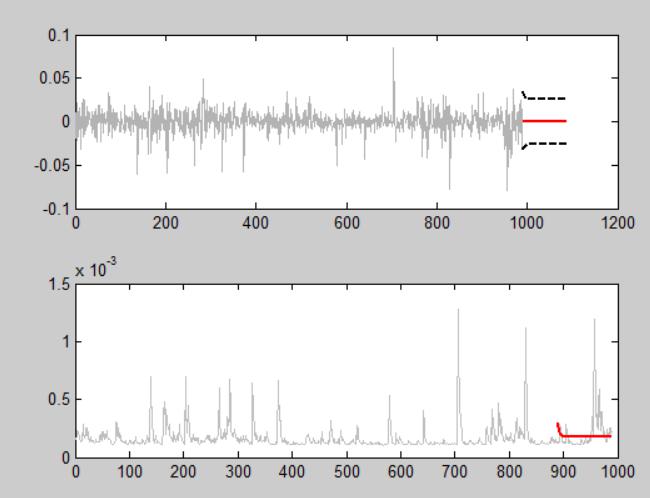
The below figure shows the predictability of the GARCH(1,1) model. The bottom panel shows that the conditional variance seems to be estimated well through a GARCH model. However, the upper panel still shows the failure of the GARCH model in estimating the mean of the process.analysis techniques代写
-
Case 2: IBM.N
The procedure of GARCH modelling for the IBM.N is similar to that of the JPM.N data. According to the ACF and PACF plot below, the result is very similar to that of the GARCH model of JMP.N.analysis techniques代写
Conditional variance and standardized residuals of GARCH(1,1):
Conditional variance and standardized residuals of GARCH(1,1) are plotted as followings. It is easy to see that the conditional variance of the residuals, or more particularity, the conditional validity has a high persistency. That is, the momentums of the conditional variance are able to keep several days. The bottom panel of the above figure shows the standard residuals. The standard residual is very likely to be a white noise process.analysis techniques代写
However, the volatility of IMB.N seems to have more picks than that of JPM.N, even though the high persistency still can be found in the above figure. The reason might be the property of IMB, a technology company, influences the log return of the stock price has more picks in conditional variance.
The below figure shows the predictability of the GARCH(1,1) model. The upper panel still shows the failure of the GARCH model in estimating the mean of the process. The bottom panel shows that the conditional variance seems to be estimated poorly through a GARCH model. However, the
VAR modeling
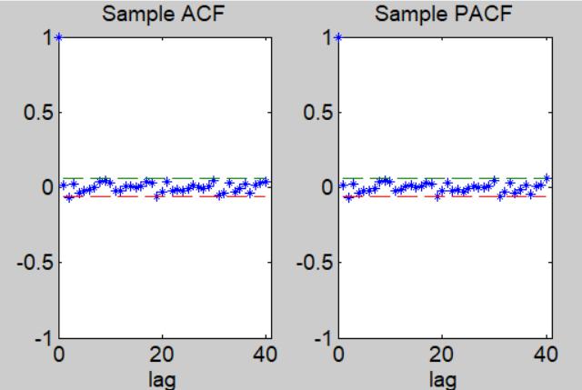
For modeling the two time series data sets jointly, A VAR mdeol is applied. The ACF and PACF of the vector time series are shown as below.analysis techniques代写
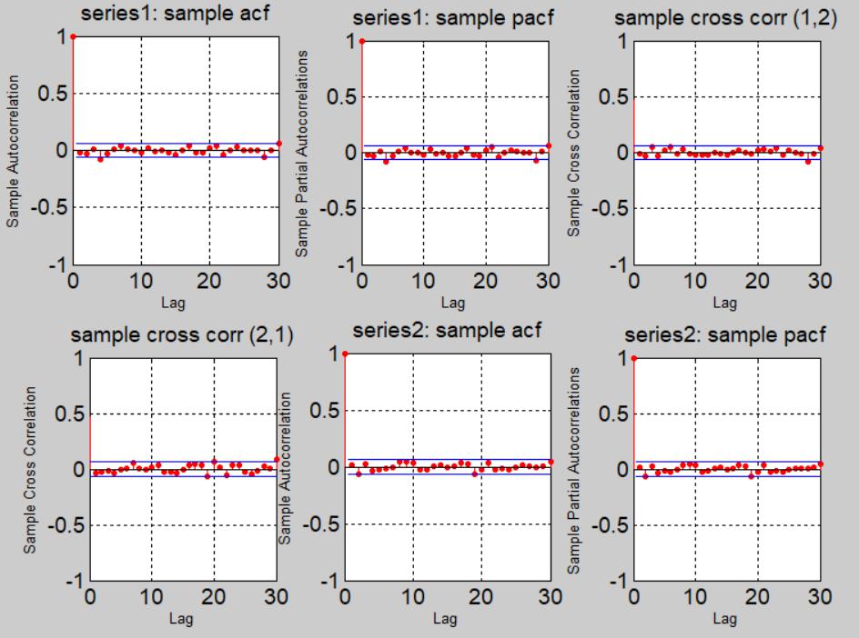
The above figure suggests a VAR(1) model might be useful for such jointly modeling. The further result shown in code also suggest a VAR model is able to model the cointegration as well as the conditional volatility for this data set.
