
Case Study: Heavy-Tailed Distribution and Reinsurance Rate-making
会计案例研究代写 The purpose of this case study is to give a brief introduction to a heavy-tailed distribu- tion and its distinct behaviors in contrast with
October 28, 2016
The purpose of this case study is to give a brief introduction to a heavy-tailed distribu- tion and its distinct behaviors in contrast with familiar light-tailed distributions in standard texts. You will learn about QQ-plot, which is a popular tool for checking goodness-of-fit for a particular statistical model. You will also work on a real-life application of heavy-tailed distributions in reinsurance rate-making.会计案例研究代写
Reinsurance is a very important component of the global financial market. It allows insurers to take on risks that they would otherwise not be able to. Did you know that NASA buys insurance contracts for every rocket it launches and every satellite and probe it sends to the outer space? These equipments are so expensive that typical insurers would not be able to cover on their own. Therefore, they can go to the reinsurance market,slide up the coverage and transfer partial coverage to reinsurers that exceed their financial capabilities. By the end of this case study, you will be able to learn basic principles of pricing an reinsurance contract.
Learning Objectives:
- Visualize the concepts in the Central LimitTheorem;
- Identify cases where the Central Limit Theorem does notapply;
- Reinforce the concept of cumulative distributionfunction;
- Understandwhy and how QQ-plot works for the assessment of goodness-of-fit;
- Reinforce the concepts of conditional probability and conditionalexpectation;
- Apply basic integration technique to compute mean excessfunction;
- Learn about behaviors of a heavy-taileddistribution;
- Learn how to use order statistics to estimate quantiles and mean excessfunction;
- Develop intuition behind point
1 Background 会计案例研究代写
1.1 Central limit theorem
This section is to provide visualization of central limit theorem which you should already be familiar with. We provide examples on both discrete random variable and continuous random variable.
Example 1.1.
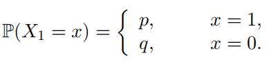
(Bernoulli random variables) Suppose we intend to test the fairness of a coin, i.e. whether the coin has equal chance of landing on a head or a tail. We can do so by counting the number of heads in a sequence of coin tosses. The number of heads in each toss is a Bernoulli random variable, denoted by X1. Let p be the probability of a head and q = 1 − p be the probability of a tail. Then, its probability mass function is given by
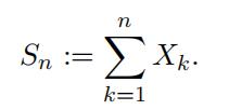
We let Xk be the number of heads in the k-th coin toss, k = 1, 2, · · · , n. Then we count the total number of heads after n coin tosses.
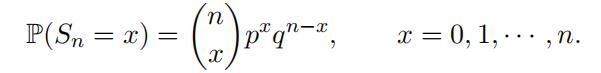
Then it is easy to show that Sn is a binomial random variable with parameters n and p
and its probability mass function is given by
For example,
suppose that we have an unfair coin with p = 0.3. Figure 1 shows the probability mass functions of the number of heads, Sn, where the number of coin tosses n = 1, 2, 3, 10, 20, 50. Since p < 0.5, we are more likely to see a smaller number of heads than that of tails in any given n tosses. In general, the probability mass function of Sn tends to skew towards to the right. However, as one can see in the later graphs in Figure 1, the probability mass function becomes more and more symmetric1 as n gets bigger and bigger. This phenomenon is present for any p ∈ (0, 1), no matter how extreme is p. Why is this happening? The answer is the Central Limit Theorem, which we have already learned in class.会计案例研究代写
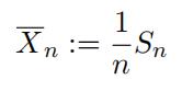
Let us consider the sample average
1Note, however, this is not to suggest that the coin becomes fair.
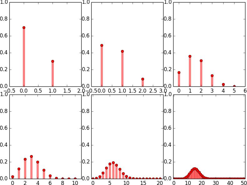
Figure 1: Probability mass function of Sn
Since the expectation of the sample average
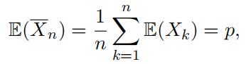
the sample mean provides an unbiased estimator of the unknown parameter of fairness p.
Exercise 1.1.
The Central Limit Theorem tells us that the estimator Xn is asymp
totically normal. In particular, we can construct the following random variable, Yn,
such that
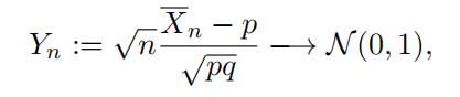
where N (µ, σ2 ) is a normal random variable with mean
µ and variance σ2 . Explain why the estimatorXn behaves roughly like N p, pq n .
[HINT: First, note that Yn is approximately N (0, 1). Now, reformulate the givenequation to express Xn as a function of Yn; what kind of function do you get?
Combine these two facts to determine the distribution of Xn by computing E(Xn)
and Var(Xn).]会计案例研究代写
As the sample size n gets big, the variance is so small that the sample average gives very good estimate of the actual parameter p. That is why in practice we use the value of Xn as an estimate, despite the fact that it is in fact a random variable.
Exercise 1.2.
What is the exact distribution of Xn?
[HINT: First, determine the set of all values of Xn that can occur. Then, note thatXn as a function of Sn, and apply the probability mass function of Sn to derive
the probability mass function of Xn. As a reminder, your probability mass function
should give P(Xn = k) for all possible outcomes of Xn. ]
Let us verify numerically the conclusion of Central Limit Theorem. Similar to what you showed in Exercise 1.2, one can show that the exact probability mass function of Yn is given by
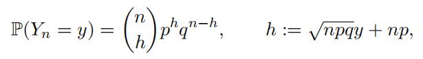
where y = (k − np)/√npq for k = 0, 1, · · · , n.
We can draw graphs of the probability mass functions and see how they converge to a normal distribution as n increases. Figure 2 below is an illustration of the central limiting theorem. The blue bars visually depict how a point mass function of a binomial random variable behave over an interval. The red dashed lines indicate the normal density function. From left to right, top to bottom we have the densities for binomial random variables with sample size n=1,2,5,20,100,1000 respectively, with probability of success being once again 30%.会计案例研究代写
Example 1.2.
(Exponential random variables) Recall that the probability density function of an exponential random variable is given by
f (t) = λe−λt, t ≥ 0
where E(Xi) = 1/λ. If we redefine Xn, Yn, and Sn according to this new random variable, then the Central Limit Theorem tells us that
Yn := √n(λXn − 1) −→ N (0, 1).
Let us compute this analytically.
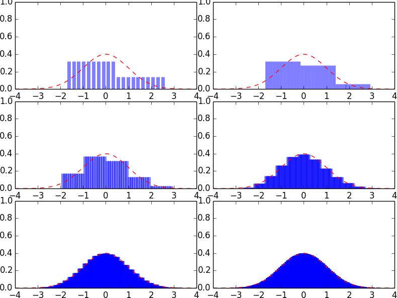
Figure 2: Binomial probability mass converging to normal density
Exercise 1.3.
It can be shown that the probability density function of Sn is given
by
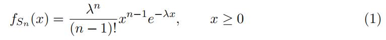
Using this density function, show that the probability density function of Yn is

both (a) the set of possible outcomes for Yn based on the set of potential outcomes
for Sn, and (b) the probability density function of Yn over these outcomes, based on
the probability density function of Sn.]会计案例研究代写
Figure 3 is a visual illustration of the probability density function of Yn for various choices of n.
We can see how the probability density function for Yn converges to the standardnormal density function. Again the red dashed lines is the standard normal density functionwhile the blue lines are the densities for Yn, given above, for n = 1, 2, 3, 5, 10, 100.
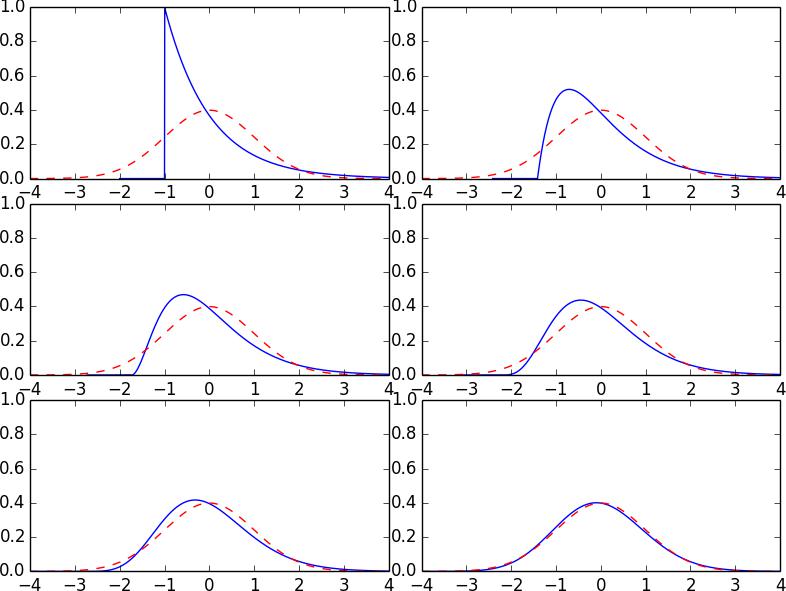
Figure 3: Exponential densities converging to normal density
Exercise 1.4.
Use matplotlib in Python to create plots showing how fYn (y) converges to the normal distribution as n increases. Your plots should contain an outlineof the normal distribution like Figure 3. Use n = 1, 2, 10.
In general, we can conclude that Central Limit Theorem tells us that the distribution of an average tends to be Normal, even when the distribution from which the average is computed is non-Normal. However, there are certain cases in which the average deviate from Normal behavior. When does the Central Limit Theorem not hold?
1.2 Heavy-tailed Distributions
Let us introduce heavy-tailed distributions which are probability distributions with a heav- ier tail than the exponential. We will see how the extremes produced by heavy-tailed distri- butions will corrupt the average so that an asymptotic behavior different from the Normal behavior is obtained. Formally, a random variable X is said to have a heavy-tailed if
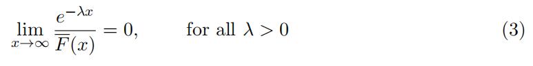
where F (x) := P(X > x) (here, F (x) is often referred to as a survival function).
An example of a heavy-tailed distribution is the Pareto distribution. Consider the strict Pareto random variable whose density is given by
f (x) = αx−α−1, x > 1
where α is a positive number, called the Pareto index. The Pareto distribution is very important in reinsurance so we will study it closely.会计案例研究代写
Exercise 1.5.
Show that the Pareto may not have fifinite mean or variance by
calculating the mean and variance of a strict Pareto random variable. Are there any
values of α for which either does not take a fifinite value?
[HINT: Examine the case when α ∈ (0, 1] and α > 1]Exercise 1.6. 会计案例研究代写
The Pareto distribution is closely related to the exponential. Given
X is a strict Pareto random variable, show that Y = ln(X) is exponentially dis
tributed with mean α 1 .
Exercise 1.7.
Using the defifinition of heavy-tailed from Equation 3, show the
following:
(a) A strict Pareto random variable is heavy-tailed.
(b) An exponential random variable with rate α is not heavy-tailed.
[HINT: You may need to apply L’Hospitˆol’s rule when taking the limit for (a). Forpart (b), consider selecting λ < α.]
2 QQ-plot 会计案例研究代写
Quantile-quantile plot, also known as QQ-plot for short, is a visual tool to check if a proposed model provides a plausible fit to the distribution of the random variable at hand. It is also a good visualization tool to see if a distribution is heavy-tailed. Let us first define what is a quantile function with an example.
Example 2.1.
(Exponential distribution) Recall the cumulative density function for ex- ponential with rate λ is given by
Fλ(x) := 1 − exp(−λx), x > 0
and the survival function of the exponential is
F λ(x) := 1 − Fλ(x) = exp(−λx), x > 0
Suppose we have real data x1, x2, · · · , xn which we suspect might be exponentially distributed with some λ > 0. We can order these observations from the smallest to the largest. Denote the i-th smallest observation by x(i).
The quantile function for the exponential function has the form
Qλ(p) = − λ ln(1 − p), p ∈ (0, 1).会计案例研究代写
Note that, of λ = 1, we have Q1(p) = − ln(1 − p). Hence, there exists a simple linear rela- tion between the quantiles of any exponential distribution and the corresponding standard exponential quantiles
Qλ(p) = λ Q1(p), p ∈ (0, 1).
Note that we do not know the exact distribution of the unknown random variable, let alone the quantile. Nevertheless, we can replace the unknown quantile Qλ by the empirical distribution Qˆn where
Qˆ (p) = x, for i − 1 < p ≤ i
In two-dimension, we essentially plotting the points with values
(− ln(1 − p), Qˆn(p))
for several values of p ∈ (0, 1). A typical choice of values of p is given by
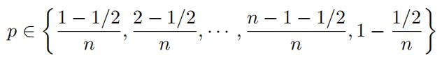
In other words, p = (j 1/2)/n for j = 1, 2, . . . , n. We then expect that a straight line pattern will appear in the scatter plot if Qˆn(p) indeed resembles Qλ(p), in other words, if the exponential model provides a plausible statistical fit for the given data set. When a straight line pattern is obtained, the slope of a fitted line can be used as an estimate of the parameter 1/λ.
2.1 Interpreting QQ-plots
The discussion in the previous section compares our observed data with the exponential distribution using QQ-plots. If our QQ-plot looks like a straight line, then our data fit the exponential distribution, since our data grow proportionally with the quantiles of the exponential distribution; in this case the specific slope of our line will depend on the rate
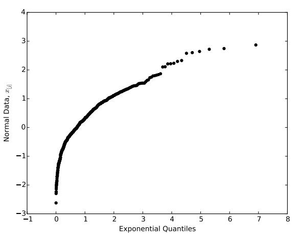
Figure 4: QQ-plot comparing normal data to an exponential distribution
λ. But what if our QQ-plot does not look like a straight line? In this case, we are not sure what distribution best fits our data, but may be able to gain some insights on how its shape differs from the exponential. Since we are interested in heavy-tailed distributions, we will focus on behavior in the tails of our distribution.
Consider the QQ-plot in Figure 4. Observe that this plot does not fit well to a straight line;
as we move from left to right, the slope of this plot decreases. First, letsfocus on the right side of the plot, which corresponds to the right tail of the distribution. If our observed data in the right tail were increasing proportionally with the quantiles of the exponential distribution, then the right portion of our QQ-plot would look line a straight line.会计案例研究代写
However,
we see that our plot is curving downward; therefore, the observations in our right tail are growing more slowly than the quantiles of the exponential distribution. This behavior suggests that our data have a lighter right tail than the exponential distribution. Now, let’s focus on the left side of our plot, which corresponds to the left tail of our distribution. As we move to the left, we see that our plot is curving downward, which suggests that our data are decreasing more quickly than the exponential distribution. This behavior suggests that our data have a heavier left tail than the exponential distribution.Together, these two facts imply that our data show a left skew when compared to the exponential distribution.
To give insight into the reason for our observations,
note that the observed data depictedin Figure 4 are taken from a standard normal population. The probability density functions of the normal and exponential distributions are depicted in Figure 5. Comparing the two, we can clearly see why the normal distribution has a heavier left tail than the exponential; the exponential distribution has a minimum value of zero, while the normal distribution can take any negative value.Comparisons in the right tail are not as clear cut, because
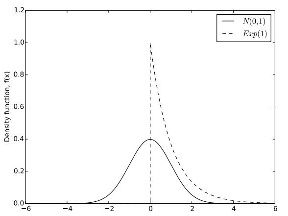
Figure 5: Probability density functions of the N (0, 1) and Exp(1) distributions
both distributions can take arbitrarily large values. However, as we look out further to the right, you can see that the exponential is larger than the normal pdf when x is non- negative. Hence, the exponential distribution has as heavier right tail than the normal distribution, since it is more likely to produce values farther to the right. Again, these two facts show that the normal distribution has a left skew when compared to the exponential.
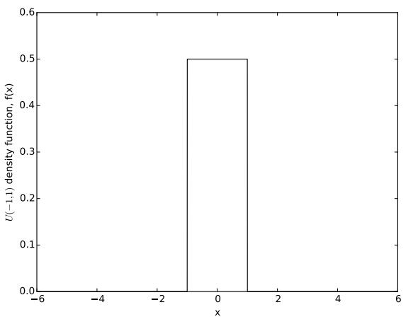
Figure 6: Probability density function of the U (−1, 1) distribution
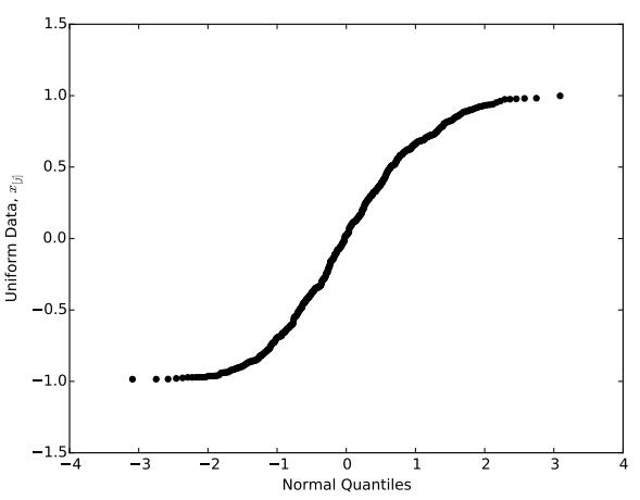
Figure 7: QQ-plot comparing U (−1, 1) data to an normal distribution
Suppose that our data were instead taken from a U (−1, 1) population, whose pdf is depicted in Figure 6. Comparing this distribution to the N (0, 1) pdf in Figure 5, we see that the U (0, 1) distribution can only generate observations between −1 and 1, while the N (0, 1) distribution can generate arbitrarily large positive and negative observations.
Hence, the N (0, 1) distribution has heavier left and right tails than the U (0, 1) distribution. To observe this fact from data, consider Figure 7, which shows a QQ-plot created by generating 500 observations from the U (−1, 1) distribution and comparing them to the normal distribution. As we look to the left, we see that the data decrease more slowly than the normal quantiles, suggesting that the normal distribution has a heavier left tail than our (uniform) data. Similarly, as we look to the right, the data increase more slowly than the normal quantiles, suggesting that the normal distribution also has a heavier right tail than our data. Hence, our conclusions from the data agree with our earlier conclusions from observing the uniform and normal pdfs.
Exercise 2.1.会计案例研究代写
Generate 500 observations from a U(0, 1) distribution, and create a QQ-plot comparing these observed data to the exponential distribution. Does you data show a heavier or lighter right tail than the exponential distribution? Create a plot of both the U(0, 1) and Exp(1) probability density functions distributions and explain why these plots support your conclusions.
Note that,
in the above discussion, we did not say that a particular distribution has a heavy tail, we only said that one distribution has a heavier tail than another distribution. To think of this another way, you would say that two sheets of paper are heavier than one sheet of paper, but it is unlikely that you would say that two sheets of paper are heavy. In our case, we say that a distribution has a heavy right tail if its tail is heavier than the exponential distribution, and has a heavy left tail if is tail is heavier than −X, where X is an exponential random variable.
Example 2.2.
Figure 8 depicts a normal QQ-plot of 100 observations drawn from a Pareto distribution with α = 3 . It shows that the sample average is far from a normal distribution. This illustrates numerically that the classical Central Limit Theorem does not apply for the Pareto distribution.
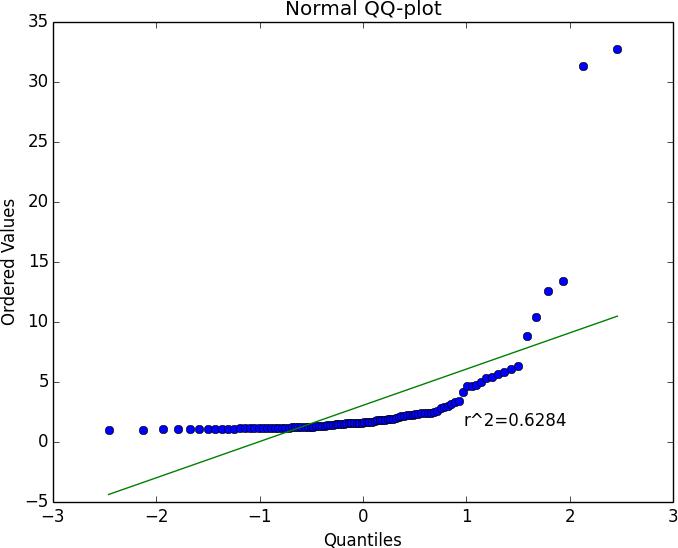
Figure 8: Normal QQ-plot for Example
Exercise 2.2.
Give a justifification why the QQ-plot in Example 2.2 fails to exhibit
a pattern of normality even with a relatively large sample size of 100. [HINT:
Consider the requirements for applying the Central Limit Theorem.]
2.2 Using real insurance claims data
Let us create a QQ-plot using real data. we investigate the insurance claim data from a reinsurance company. The data set insurance.txt contains automobile claims from 1988 until 2001 which are greater than 1, 200, 000 euro. This data set contains n = 371 obser- vations.
Exercise 2.3.
Using Python, generate the QQ-plot by doing the following:
1.Read the data and select only the largest 270 observations
2.Take a logarithmic transform of the selected observations
3.Using matplotlib and scipy.stats.probplot, create exponential and normal QQ plots of the data.
Does the data fifit an exponential or normal distribution? Justify your answer. Notethat, if the exponential provides a good fifit to your data after a logarithmic trans formation, then your result from Exercise 1.6 suggests that the data fifit a Pareto distribution.
3 Mean excess function and reinsurance 会计案例研究代写
Reinsurance is an insurance policy purchased by an insurance company from one or more other insurance companies, known as the “reinsurer”, as a means of risk management. It is a very common market practice when insurance companies undertake high risk profiles with potential catastrophic losses. A reinsurance agreement details the conditions upon which the reinsurer would pay a share of the claims incurred by the insurer and the reinsurer is paid a “reinsurance premium” by the insurer, which issues insurance policies to its own policyholders. A diagram of cash flows among the participants in an insurance market can be found in Figure 9.
A common form of reinsurance is the excess of loss (XL) reinsurance,
where the insurer covers insurance claims from policyholders up to the maximum of its retention level and any amount beyond the retention will be reimbursed by the reinsurer. For example, an insurance company might insure commercial property risks with policy limits up to $10 million, and then buy reinsurance of $5 million in excess of $5 million. In this case a loss of $6 million on that policy will result in the recovery of $1 million from the reinsurer.会计案例研究代写
The modeling of the XL reinsurance relies on an important mathematical concept, called the mean excess function. Suppose a ceding insurer enters into an XL treaty with a retention level t. Let X be a random variable governing the size of a particular policy-
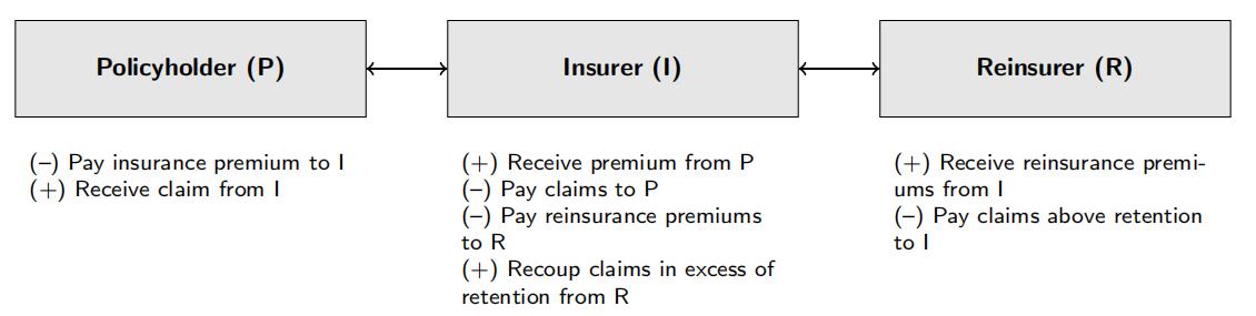
Figure 9: Participants in an insurance market
holder’s claim. After claim investigation, the ceding insurer will make the payment and the reinsurer has to pay X − t if X > t. Pricing actuaries from reinsurance companies would want to know the average cost of such claims, which is theoretically determined by the mean excess function
e(t) = E(X − t|X > t) = E(X|X > t) − t. (4)会计案例研究代写
Exercise 3.1.
Show that the mean excess function of an exponential random vari
able with mean 1/λ is given by
X > t, can be expressed as fX|X>t(x) = fX(x)/P(X > t) if X > t (and 0 otherwise),
where fX(x) is the PDF of random variable X. Apply the defifinition of expectation,
using this distribution, to compute E(X t|X > t)].会计案例研究代写
Exercise 3.2.
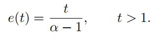
Show that the mean excess function of a strict Pareto random vari
able with the Pareto index α is given by
Observe that the mean excess function can also be written as2
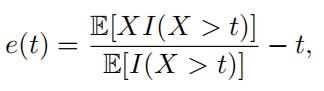
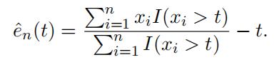
where I(A) = 1 if the event A is true and 0 otherwise. In practice, we replace the theoretical mean by its empirical counterpart. Given the sample data x1, x2, · · · , xn, the mean excess function is estimated by
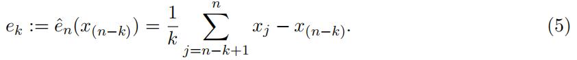
Often the empirical function eˆn is evaluated at t = x(n−k), the (k+1)-th largest observation.
Then the numerator equals Σn xiI(xi > t) = Σn xj, while the denominator equals
![]() . The estimates of the mean excesses are then given by
. The estimates of the mean excesses are then given by
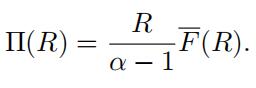
Consider an XL reinsurance contract with a retention level R. The reinsurer is obligated to pay for the claim amount in excess over the limit R. The fair net premium3 is given by
Π(R) = E[(X − R)+], (6)
where (x)+ = max{x, 0}. Equivalently, we obtain
Π(R) = e(R)F (R). (7)
Since reinsurance contracts are meant to transfer risks of catastrophic losses, claims of small and medium sizes provide no useful information for the valuation of reinsurancecontracts. Let us consider a reinsurance contract with various retention levels, for exampleR = 5, 000, 000 euro, which is typically used in practice. Observe that only 12 observations are larger than that level in the given data set. We use two methods in this case to determine the net premium.会计案例研究代写
2To see this result, note that XI(X > t) is a function of random variable X, such that XI(X > t) = X if X > t (and 0 otherwise). Hence, we can compute E[XI(X > t)] as we do any other function of X
3Net premium refers to the pure cost of insurance coverage. It is used in contrast with gross premium,which includes commission, policy expenses and other administrative costs.
Exercise 3.3.
(Estimator #1: non-parametric) The simplest way to estimate the
net premium Π(R) is to use an empirical estimator of (6) given by
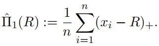
Develop a computer algorithm in Python to estimate the net premiums for various
retention levels in Table 1.
Exercise 3.4.会计案例研究代写
(Estimator #2: non-parametric) Another way to determine the net
premium is to make use of the identity (7)
ˆΠ2(R) := ˆen(R)ˆF n(R),
whereˆF n(R) is some estimator of the tail probability F(R) = P(X > R).
If R is fifixed at one of the sample points, that is, R = x(n k) , the non-parametric estimator is given by
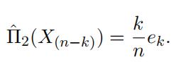
If R is not fifixed at one of the sample points, then we have to introduce an estimator
for F(R). There are many difffferent ways of defifining an estimator. For example, one can estimate F(R) as
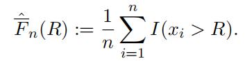
Substituting this back into our estimator ofˆΠ2(R), we find
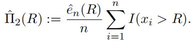
Show that, if we defifineˆΠ2(R) in this way,
then this estimator for the net premium is the same asˆΠ1(R). [HINT: You should be able to demonstrate that these are equal by algebraic manipulation.]
Note that in the previous two pricing models we did not use any assumption of a parametric model. As much as we prefer simplicity, we should also keep in mind a general rule from statistical theory that statistical estimators do not provide accurate results whenthe size of sample data for estimation is very small. When R = 5, 000, 000 euros, only 12observations enter into the calculations of Πˆ1 and Πˆ2. It is essentially a waste of information from other data points below 5 million eurors.
We learned from Exercise 2.3 that Pareto distribution provides a good fit for the large observations in the data set.
Hence, we should take advantage of this extra information extracted from the data set. One should keep in mind, however, that the strictly Pareto fits the large observations well but not necessarily for small data points. It indicates that the data set can be modeled by a Pareto-type distribution, whose tail behaves like a Pareto distribution. Without getting into too much technical details regarding Pareto-type distributions, we consider a scaled Pareto distribution for our analysis. Suppose the large observations all came from a random variable X, whose survival probability function is given by
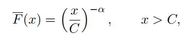
for some large number C > 0. It means that X is C times a strictly Pareto random variable.Hence it is easy to show that the mean excess function of the scaled Pareto random variable remains the same as in Exercise 3.2. This indicates that we can get around estimating the constant C when using estimates of the mean excess function.
Hence it remains to estimate the unknown parameter α,
whose reciprocal, γ := 1/α, is known as the extreme value index, in the extreme value theory. A well-known estimator of the extreme value index, called the Hill estimator, was proposed in Hill [1]. The intuition behind this estimator can be easily explained. It follows from Exercise 1.6 and Exercise 3.2 that the mean excess function of the logarithmic of the strict Pareto random variable (and that of the scaled Pareto random variable) is 1/α. According to (5), it would be natural to consider
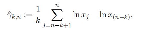
This is the Hill estimator. It enjoys a high degree of popularity thanks to some nice theoretical properties, which we do not intend to discuss in this class. For example, it has been proven that the Hill estimator is a consistent estimator for γ. (https://en. wikipedia.org/wiki/Consistent_estimator) One should note that the Hill estimator is based on k-largest observations and for each choice of k there would be an estimate of γ. Many researchers have developed strategies to determine the optimal k under variousstatistical criteria. The discussion of such procedures can be quite evolved and hence should be omitted here.
Exercise 3.5.
(Estimator #3: parametric) By combining our result from Exercise
3.2 with equation 7, we can also write
If the retention level R is situated within the sample, say R = x(n k) , then we can
use the estimator
If R is not fifixed at one of the sample points, then we have manipulate the net
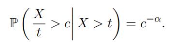
premium formula to adopt a difffferent form. By applying the defifinition of conditional probability with c > 1, we can show that
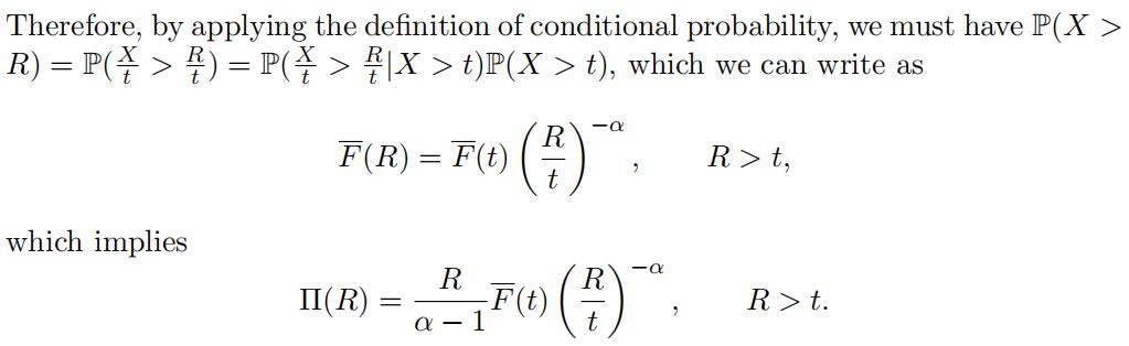
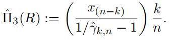
Let k be an appropriate choice for the number of largest observations and set t =x(n k) .
It we estimate α as the inverse of the Hill estimator and estimate F(x(n k))
as k/n, another estimator of net premium is given by
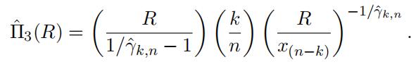
Suppose the optimal choice of k is 95. Compute the estimators in Table 1 based on the parametric model.
Now you have completed a pricing exercise that an actuary would typically do for an reinsurance contract on luxury commodities. You can see that there is no “one-size-fits- all” magic formula for pricing a product. Keep in mind that each of the estimators we developed has its own merits and limitations. Observe from your solutions to Table 1 that the estimates of net premiums are close for small rention levels, as more data are used in all
| R | Πˆ1 | Πˆ3 |
| 3,000,000 | ||
| 3,500,000 | ||
| 4,000,000 | ||
| 5,000,000 | ||
| 7,500,000 |
Table 1: Estimates for Π(R)
estimators. But they are far apart for high rention levels, due to the “low quality” results from the non-parametric statistics with limited sample data. An advanced knowledge of heavy-tailed distribution allows us to have better use of data information and provide more trust-worthy solutions in this example, which would be very important for billion-dolloar businesses like reinsurance.
References
[1] Hill, B.M. (1975). A simple approach to inference about the tail of a distribution.Annals of Statistics. 3: 1163–1174.

其他代写:考试助攻 计算机代写 java代写 function代写 paper代写 web代写 编程代写 report代写 数学代写 algorithm代写 python代写 java代写 code代写 project代写 Exercise代写 dataset代写 analysis代写 C++代写 代写CS 金融经济统计代写 作业帮助
