LECTURE NOTES
OPTIMIZATION代写 Abstract. These are lecture notes for co255 in the Fall 2019 term.Topics covered:(1)Linear Optimization, Convexity (4 weeks)
FOR CO255 INTRODUCTION TO OPTIMIZATION
FALL 2019
LEVENT TUNC¸ EL
Abstract. These are lecture notes for co255 in the Fall 2019 term.
Topics covered:
- Linear Optimization, Convexity (4 weeks): Duality in linear optimization. Farkas’ Lemma and the theorems of the alternative. Duality theorem for linear programming. Complementary Slackness theorem. Simplex Method. Polyhedra and elementary convex
- Combinatorial Optimization (4 weeks): Linear diophantine equations. Facets of polyhedra. Integrality of polyhedra. Shortest paths and optimal flows. Total Unimodularity. K˝onig’s Max. Flow-Min. Cut Theorem. (Hungarian) Bipartite matching algorithm.OPTIMIZATION代写
- Continuous Optimization (4 weeks): Convex functions. Analytic characteri- zations of Existence and uniqueness of optimal solutions. Separating and supporting hyperplane theorems. Lagrangian Duality. Karush-Kuhn-Tucker Theorem. Conic Optimization problems. EllipsoidMethod.
Date: Fall 2019. October 21, 2019.
Department of Combinatorics and Optimization, Faculty of Mathematics, University of Waterloo, Waterloo, Ontario, N2L 3G1, Canada (e-mail: ltuncel@math.uwaterloo.ca).
Contents OPTIMIZATION代写
1.OpeningRemarks 3
2.Farkas’ Lemma and the Theorems ofthe Alternative 3
2.1Some opening historical remarks forLinear Optimization 3
2.2Fourier’s Approach to Solving Systems of Linear Inequalities 10
2.3Example of Fourier Elimination withTwo Variables: 11
3.Duality Theorems forLinear Optimization 17
3.1WeakDuality Relation 19
3.2StrongDuality Theorems 20
3.3Complementary Slackness Conditionsand Theorems 22
3.4Duals of LP Problems inGeneral Forms 25OPTIMIZATION代写
3.5General Recipe for theDual Problem 25
4.Polyhedra and ElementaryConvex Geometry 28
4.1Extreme Points of Convex Sets, Internal Structureof Polyhedra 31
4.2Polytopes 33 OPTIMIZATION代写
5.SimplexMethod 36
5.1Lexicographicsimplex method 42
5.2StrictComplementarity Theorem 48
6.CombinatorialOptimization 50
1.OpeningRemarks
This course will provide an introduction to optimization together with a strong foun- dation to continue with more advanced undergraduate work, graduate work as well as research work.OPTIMIZATION代写
We will make a mathematical introduction to various topics in optimization in this high-pace, theoretically oriented course. Successful completion of this course would satisfy most of the prerequisites for all 400, 400/600 level optimization courses in C&O. Those are co45*, co46*, co47*.
2.Farkas’ Lemma and the Theorems of theAlternativeOPTIMIZATION代写
2.1Some opening historical remarks for Linear Optimization.
The history of Linear Optimization (or Linear Programming) is connected to various areas of math- ematics, operations research and mathematical economics.The applications (both in practice and theory) are far reaching and are significantly beyond the disciplines where it originated.OPTIMIZATION代写
George B. Dantzig [1914–2005] is widely admired as the Father of Linear Programming. He proposed the Simplex Method in the 1940s. See his seminal book on the subject [?]. Dantzig’s father, T. Dantzig, was also a mathematician who worked with Henri Poincar´e. George Dantzig completed his Ph.D. with J. Neyman (recall Neyman-Pearson Lemma in Statistics) at UC Berkeley.OPTIMIZATION代写
The name Programming in Linear Programming does not refer to computer program- ming. When Dantzig was working for the U.S. Air Force at the Pentagon during the late 1940s, he was trying to mechanize (his choice of the word) the preparation of plans to move troops, supplies, training etc. At that time in the military terminology, program- ming meant preparing plans and proposed schedules. (They used computer code as we still do to refer to software.)
Together with Dantzig,
two other main contributors, John von Neumann [1903–1957] and Leonid Kantorovich [1912–1986] stand out as the main founders of the theory of linear optimization in the first half of the 20th century.
Linear Programming (LP) problem can be defined as the problem of optimizing (mini- mizing or maximizing) a linear function of finitely many real variables subject to finitely many linear equations and inequalities.OPTIMIZATION代写
Since the 1940’s Simplex Method has been a great success in all fronts: theory, appli- cations and efficient computations. Many variants of Dantzig’s original algorithm have been proven to have the finite termination property, many successful pivot rules for gen- eral LP problems and for special ones, e.g. network flow problems, have been proposed and studied in some detail. Very many practical problems, from production scheduling to managing oil refineries, have been successfully modeled as LP problems and solved by variants of the simplex method.
On the theoretical side,OPTIMIZATION代写
many extensions to multi-objective optimization, nonlinear pro- gramming etc. created very important fields. In the mid 1960’s and the early 1970’s there was a great deal of interest sparked by some optimizers and some theoretical computer scientists. The interest was in classifying computational problems as relatively easy and relatively hard with respect to some sound mathematical framework. As these thoughts led to the development of the theory of NP-completeness and many deep extensions, the optimizers wanted to know whether the most commonly known optimization problem Linear Programming was solvable in polynomial-time or not. As a result, LP played an important role in inspiring research work in Computational Complexity and to date it con- tinues to be very influential in the theory and practice of various areas in Mathematics, Statistics and Computer Science, in addition to its obvious impact on applications.
Theorem 1. (Fundamental Theorem of Linear Algebra) Let A ∈ Rm×n, b ∈ Rm be given. Then exactly one of the following systems has a solution:
- Ax =b;
- ATy = 0, bTy ƒ=0.
Notes:
- Wemay replace bTy ƒ= 0 with bTy = −1 (or any other non-zero constant) because y can be scaled as needed to match any constant.
- Forthis course, every vector is assumed to be a column
- Since every operation requires appropriately dimensioned vectors, when it is not statedexplicitly the vectors’/matrices’ dimensions can be assumed to For example the 0 vector in ATy = 0 above must be n dimensional.
- All equalities and inequalities mean all elements of the vector/matrix hold equal- ity/inequality simultaneously.OPTIMIZATION代写
An alternate statement (with a geometric interpretation below) of the Fundamental Theorem of Linear Algebra is as follows:
Let A ∈ Rm×n, b ∈ Rm be given. Then exactly one of the following statements is true:
(I)b ∈Range(A);
(II)∃a vector in Null(AT) which makes a nonzero inner product with b.
The above is an equivalent statement to the original Fundamental Theorem of Linear Algebra. By definition, b ∈ Range(A) (range is also known as column-space, and means the set of vectors composed by a linear combination of the columns of matrix A) iff ∃ x such that Ax = b. Similarly, in (II), by definition of the nullspace (the set of vectors x such
that Ax = 0) the statement is essentially a rewritten version of the original theorem. This alternate version is particularly interesting because geometrically if b can be expressed as a linear combination of columns of A then we clearly have a solution (the coefficients of the linear combination), and when b cannot be expresses only as a linear combination of the columns of A then the orthogonal projection of b onto the nullspace of AT is nonzero and the inner product of this projection (which is our y in this context) with b would also be nonzero.OPTIMIZATION代写
There are constructive proofs (proofs which give algorithms) for this theorem,
for ex- ample a careful implementation of Gaussian elimination. After the row reduction stage we would have enough information to either solve the system or recover a certificate of infeasibility.
Fundamental Theorem of Linear Algebra has the following analogue for the linear sys- tems which include linear inequalities:
Theorem 2. (Farkas’ Lemma) Let A ∈ Rm×n, b ∈ Rm be given. Then exactly one of the following systems has a solution:
(I)Ax = b, x ≥0;
(II)ATy ≥ 0, bTy <0.
In the above statement, we may replace “bTy < 0” by “bTy = −1” or by “bTy ≤ −1.” The above result is deeply connected to linear optimization. Let’s start with an example: Consider the following two-person zero-sum game. There are two players: ρ and γ. ρ secretly chooses a strategy (a number) i ∈ {1, 2} and γ secretly chooses a strategy (anumber) j ∈ {1, 2, 3}. Both players simultaneously reveal their strategies i and j. Basedon these values they pay each other the following amounts (below given 2-by-3 matrixdenotes payments in dollars to the player γ by ρ):
10 −30 40
−25 60 −40
If ρ chooses 1 and γ chooses 2 , from the matrix above the payout is -30, meaning that γ pays ρ, 30 dollars.OPTIMIZATION代写
Since we know that both players are very smart,
we will apply a ’mixed strategy’ for player γ. Player γ chooses j with probability xj. So if ρ chooses 1, γ will receive 10x1 − 30x2 + 40x3 dollars. If ρ chooses 2, γ will receive −25x1 + 60x2 − 40x3 dollars. Thus, γ wants to maximize the minimum of {10x1 − 30x2 + 40x3, −25x1 + 60x2 − 40x3}.Introduce the new variable x0. γ’s problem becomes:
Maximize x0
subject to: 10x1 − 30x2 + 40x3 ≥ x0,
−25x1 + 60x2 − 40x3 ≥ x0, x1 + x2 + x3 = 1,
x1 ≥ 0,
x2 ≥ 0,
x3 ≥ 0.
The other player, ρ’s problem is:
Minimize y0
subject to: 10y1 − 25y2 ≤ y0,
−30y1 + 60y2 ≤ y0,
40y1 − 40y2 ≤ y0, y1 + y2 = 1,
y1 ≤ 0,
y2 ≤ 0.
Let us generalize the above game to an arbitrary number of strategies for each player. Fix integers m, n ≥ 2. m is the number of strategies (moves) for ρ and n is the number of strategies for γ. An m-by-n matrix A, completely known to both players, determines thepayoff to γ by ρ. (The negative entries denote the payment to ρ by γ—recall the term zero-sum game.) The matrix A is called the payoff matrix.
Similar to the above,
ρ secretly chooses a strategy (a number) i ∈ {1, 2, . . . , m} and γ secretly chooses a strategy (a number) j ∈ {1, 2, . . . , n}. Both players simultaneouslyreveal their strategies i and j. As a result, ρ pays γ, aij dollars. (Again, if aij < 0, then γ pays ρ, −aij dollars.)
Note that the model has applications way beyond two people gambling with their money. For example, each player may correspond to a company in a given sector, i ∈{1, 2, . . . , m} and j ∈ {1, 2, . . . , n} may represent the marketing and or pricing strategies for the respective companies. Alternatively, players may represent governments, i ∈{1, 2, . . . , m} and j ∈ {1, 2, . . . , n} may represent some diplomatic strategies (and/or other moves) for the respective governments.
Let us assume that the players engage in this game many many times and let xj denote the probability that γ plays j. We want to compute the optimal mixed strategy for γ.(To maximize her winnings, how often should she play strategy j?) Then x ∈ Rn and nj=1xj = 1. Assuming ρ is smart, we can expect that ρ will choose the strategy for himself that is the best for him in this situation:
argmini {(Ax)i} .
Therefore, γ’s problem is to maximize this minimum value which can be expressed as a linear optimization problem:
max x0
s.t.
−1x0 + Ax ≥ 0,
1Tx = 1,
x ≥ 0,
where we denoted by 1 the vector of all ones of appropriate dimension (size m or n
depending on the context here).
min y0
s.t.
−1y0 + ATy ≤ 0,
1Ty = 1,
y ≥ 0
which is ρ’s problem for the same game! Hence the connection between LP duality theory and Game Theory for Two-Person Zero-Sum Games.
2.1.1Somefurther historical remarks.
Just as Dantzig was developing his ideas on Linear Programming, independently of Dantzig, von Neumann was working on Game Theory.
The first meeting between Dantzig and von Neumann is well covered in the literature, including an account of it by Dantzig himself.
Game Theory had many excited supporters; however, there were also a few who were very critical of its assumptions. Mathematician Norbert Wiener [1894-1964] who is con- sidered a founder of cybernetics was also a kind of a nemesis of John von Neumann [1903-1957]. Perhaps in our 21st century language, they were frenemies. Wiener pro- moted a continuous and analog view of the World. von Neumann, although famous for many variational results, seems to have favored discrete and algebraic approaches more in his work and his mathematical modelling. Apparently, Wiener once criticized von Neumann’s work in Game Theory by stating: “von Neumann’s picture of a player as acompletely intelligent, completely ruthless person is an abstraction and a perversion of the facts.”
2.1.2Definition of Linear Programming (LP) problems.
The above example is a linear programming problem(LP).
A function f : Rn → R is called an affine function, is there exist a ∈ Rn and α ∈ R such that f (x) = aTx + α. An affine function is linear if α = 0.
A linear constraint is any of the following
f (x) ≤ g(x)
f (x) = g(x)
f (x) ≥ g(x),
where f, g are affine functions. (The first and the last are linear inequalities; the middle one is a linear equation.)
We are ready to define the set of optimization problems called Linear Programming problems.
Linear Programming (LP) problem is the problem of optimizing (maximizing or min- imizing) an affine function of finitely many real variables subject to finitely many linear equations and linear inequalities on these variables.
Note that the inequalities are never strict inequalities, so ≤ would be used, not <. At certain points in our discussion we will address strict inequalities as well; but, if some strict inequalities are present, the optimization problem is not an LP. As we develop the theory, we will mostly focus on LP problems in
(1)standard inequalityform
Max cTx
s.t. Ax ≤ b,
x ≥ 0,
(2)standard equalityfrom
Max cTx
s.t. Ax = b,
x ≥ 0,
where A ∈ Rm×n, b ∈ Rm, and c ∈ Rn. Every LP problem can be put into the above forms.
x¯ ∈ Rn satisfying all constraints is called a feasible solution. A feasible solution xˆ ∈ Rn such that it has the best objective value among all feasible solutions, is called an optimal solution. E.g., for the maximization problems above, it is a xˆ feasible in the corresponding problem such that cTxˆ ≥ cTx, ∀ feasible solutions x.
For the problems in standard equality form, we will typically assume rank(A) = m.
This assumption can be made without loss of generality, for solving LP problems. (We first solve the linear system of equations Ax = b. If rank(A) < m, then either Ax = b has no solution—then the LP is infeasible—or we find all the linearly dependent equations inAx = b and eliminate them; we then have a linear system A˜x = ˜b whose solution set isthe same as that of Ax = b and A˜ has full row rank.)
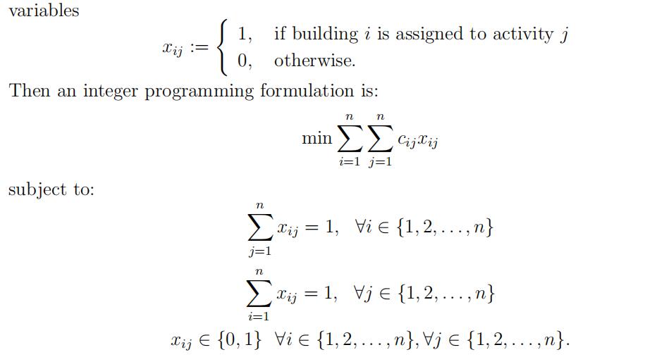
2.1.3.An Integer ProgrammingProblem.
Integer Programming (IP) problems are ob- tained from LP problems by requiring a nonempty subset of variables to be integers. InIP formulations in addition to the linear constraints (as defined above), we allow the following:
xj ∈ Z, x ∈ Zn, xj ∈ {0, 1}, x ∈ {0, 1}n.
As an example, consider the following problem:
A new university, SPIT (Smart People’s Institute of Technology), was established near the North Pole. Even though the buildings have been used for only a few years, because of the harsh weather conditions there is a need for renovation. The university planning committee is to decide on how to assign three functions (laboratory, library, tennis courts) to three available buildings (Building A,B,C). Cost of renovation for each of the nine possible matches of a building with a function/activity is given below (in millions of dollars):
| Lab | Lib | Tennis Co | |
| Building A | 6 | 1 | 2 |
| Building B | 7 | 6 | 5 |
| Building C | 6 | 2 | 4 |
How can the university planning committee assign functions to the buildings so as to minimize the total renovation cost?
Let’s generalize to n buildings and n functions (for a given integer n ≥ 3). Let cij
denote the given cost for renovating building i to serve the function/activity j. We define
2.1.4.A Nonlinear ProgrammingProblem.
Consider Fermat’s Last Theorem: There do not exist positive integers x, y, z and an integer n ≥ 3 suchthat
xn + yn = zn.
Next consider a nonlinear optimization problem with four variables:
inff (x1, x2, x3, x4) := (xx4 + xx4 − xx4 )2+(sin(πx1))2+(sin(πx1))2+(sin(πx1))2+(sin(πx1))2 subject to:
x1 ≥ 1, x2 ≥ 1, x3 ≥ 1, x4 ≥ 3.
It is not difficult to prove that the infimum above (the optimal value of the nonlinear programming problem) is zero. However, proving that this optimal value is not attained is equivalent to proving Fermat’s Last Theorem.
2.2Fourier’s Approach to Solving Systems of Linear Inequalities.
Let’s go back to studying LP problems. How do we determine whether an LP has a feasible solution? Itturns out that the question is essentially equivalent to solving for an optimal solution.
Without loss of generality, we may assume our system is Ax ≤ b, with A ∈ Rm×n, b ∈ Rm.
Next, we ask: Can we eliminate a variable? If we can, and generate another system of linear inequalities, we might be able to keep reducing the number of variables until we end up with a trivial problem to solve.
Notable work on solving systems of linear inequalities goes back at least to Joseph Fourier (recall Fourier series and Fourier transform) [1768–1830]. Fourier’s paper from 1826 addresses systems of linear inequalities. Related work of Theodore Motzkin [1908– 1970] in 1936 popularized the results. Fourier elimination eliminates the variables one at a time, incurring a potential cost of roughly squaring the number of linear inequalities in the worst-case. Most importantly, these results lead to a finite algorithm for solving systems of linear inequalities and in the case that the original system is infeasible, the method provides an infeasibility certificate (as in Farkas’ Lemma).
Let A ∈ Rm×n, b ∈ Rm be given. Suppose we want to solve the system of linear inequalities
Ax ≤ b.
Here, solving means either find xˆ ∈ Rn such that Axˆ ≤ b or prove that Ax ≤ b is not solvable. The main idea is to focus on one variable at a time, say xn, and eliminate it by possibly introducing many linear inequalities so that the new system is feasible iff the old system was.
To this end, let J− ⊆ {1, 2, . . . , m} denote the index set of the original inequalities in which the coefficient of xn is negative. Let J+ ⊆ {1, 2, . . . , m} denote the index set of the original inequalities in which the coefficient of xn is positive. (For the sake of simplicity of our presentation, we assume J− ƒ= ∅ and J+ ∅.) Let J0 denote the index set of the remaining inequalities.
By definition, xn does not appear in the inequalities indexed by J0. Then the role of xn in the original system is completely explained by
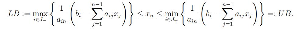
Now,
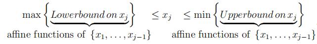
we can conclude that the original system is feasible iff there exists an assignment of values to x1, x2, . . . , xn−1 such that LB ≤ U B and all the inequalities in J0 are satisfied. The latter two conditions only involve the variables x1, x2, . . . , xn−1. So, if we can express the condition LB ≤ U B as a finite system of linear inequalities on these (n − 1) variables, then we are in business!
Indeed, this is possible. For each pair (A, k) for A ∈ J− and k ∈ J+, we write the inequality

This leads to a linear system of (|J0| + |J−| · |J+|) inequalities in (n − 1) variables. Continuing with this idea, we can reduce the initial system to a system of linear inequalities on a single variable for which both LB and U B become constants that we can compute. Note that each new linear inequality generated by this method is a nonnegative linear combination of the linear inequalities in the original system. Thus, if we find at the end that LB > U B, this observation leads to an algebraic proof of infeasibility of the original system.
2.3. Example of Fourier Elimination with Two Variables:
Ax ≤ b
is give below:
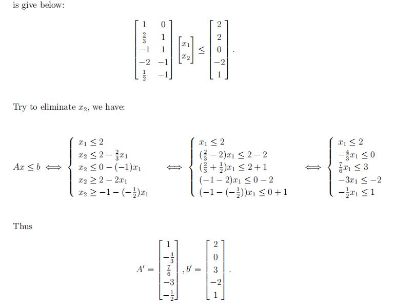
So, using one step of Fourier Elimination, we start with a linear system of inequalities Ax ≤ b in n variables and produce a system of linear inequalities Ajxj ≤ bj in (n − 1) variables. In particular, in the above example we have 2 ≤ x1 ≤ 2, thus a feasible solution to the original system of inequalities is x¯ = (1, 0)T.
In general, we have
Lemma 3.
The system Ax ≤ b is feasible iff Ajxj ≤ bj is feasible. Moreover, every feasible solution (x¯1, x¯2, …, x¯n−1)T of Ajxj ≤ bj can be extended to a feasible solution (x¯1, x¯2, …, x¯n−1, β)T of Ax ≤ b, for some β ∈ R .
Proof. We proved above in deriving the system Ajxj ≤ bj that every linear inequality in the new system is a consequence of linear inequalities of the original system Ax ≤ b. (The inequalities in J0 are identical to those in Ax ≤ b, the inequality indexed by (A, k) in Ajxj ≤ bj is a nonnegative linear combination of inequalities indexed A and k in Ax ≤ b.) Thus, “Ax ≤ b is feasible” implies Ajxj ≤ bj is.
For the converse, note that in the above derivation, the solution set of Ax ≤ b and the solution set of the following system
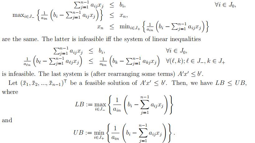
In the above definitions, if J− is empty, then LB := −∞ and if J+ is empty, then U B := +∞. In any case, since the interval [LB, U B] ∩ R is not empty, we can pick any β ∈ [LB, U B] ∩ R. Q
Remark 4. (Fourier Elimination)
Suppose we are given A ∈ Rm×n, b ∈ Rm, and we want to solve for Ax ≤ b (system of linear inequalities). Fourier Elimination partitions the index set {1, 2, . . . , m} of the rows, into J0, J+, J−, and generates a new system of linear inequalities eliminating xn.
(1)For each step of Fourier Elimination wewould compute
So, in each iteration, we have
LB(x1, x2, . . . , xj−1) ≤ xj ≤ U B(x1, x2, . . . , xj−1),
with the convention that at such an iteration, is J+ is empty, then U B := +∞ and if J− is empty then LB := −∞. If the system has a solution, then we will end up in the last iteration with the trivial system of linear inequalities
LB ≤ x1 ≤ U B,
where U B ≥ LB. Therefore, setting x1 to any value in [LB, U B] ∩ R will solve this system. So, we choose such a value for x1, call it x¯1 and go to the previous iteration. Now we plug in the value x¯1 and end up with another trivial system:
LB(x¯1) ≤ x2 ≤ U B(x¯1).
We choose x¯2 ∈ [LB(x¯1), U B(x¯1)] ∩ R and continue . . .
choose x¯j ∈ [B(x1, x2, . . . , xj−1), U B(x1, x2, . . . , xj−1)] ∩ R
… until we have the whole x¯. (Note that we have been applying Lemma 3.)
(2)In the new system of inequalities, all the new rows generated are nonnegative linear combinations of previous rows. In particular, the inequality generated from A ∈ J−and k ∈ J+ in the first iteration, is precisely 1 .the Ath row of Ax ≤ bΣ + 1 .the kth row of Ax ≤ bΣ .
Moreover,
nonnegative linear combination of nonnegative linear combinations of the system Ax ≤ b is a nonnegative linear combination of the system Ax ≤ b. Let’s verify. Let u, v ∈ Rm and consider the linear inequalities
and
uTAx ≤ uTb
Further let α, β be nonnegative real numbers. Then, the inequality
αuTAx + βvTAx ≤ αuTb + βvTb
is
wTAx ≤ wTb,
where w := αu + βv. Since u, v are both nonnegative vectors and since α and
β are nonnegative real numbers, w is a nonnegative vector and hence, the linear inequality
αuTAx + βvTAx ≤ αuTb + βvTb
is a nonnegative linear combination of inequalities in Ax ≤ b.
Therefore, every new inequality generated during a run of Fourier Elimination can be expressed as wTAx ≤ wTb for some w ∈ Rm.
(3)As in Gaussian Elimination, the computation of Fourier Eliminationcorresponds to pivoting of rows. In Gaussian Elimination we can use any number as the coefficient of the linear combination, however in Fourier Elimination we restrict ourselves to positive numbers to preserve the direction of inequality.
Theorem 5.
Let A ∈ Rm×n and b ∈ Rm. Then, exactly one of the following has a solution:
(I)Ax ≤b;
(II)ATu = 0, u ≥ 0and bTu < 0.
Proof. Suppose that both systems have solutions (we are seeking a contradiction). That is, ∃x¯ ∈ Rn such that Ax¯ ≤ b, and ∃u¯ ∈ Rm, u¯ ≥ 0 such that ATu = 0 and bTu < 0.
Claim 1. (I) and (II) cannot both have solutions.
A contradiction!
Therefore, (I) and (II) cannot both have solutions.
Claim 2.
¬(I) ⇒ (II) Suppose (I) has no solution, then we apply Fourier Elimination to Ax ≤ b. By the last lemma and Remark 4. part (2), at the last iteration of Fourier Elimination we obtain the following inequality:
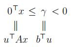
After we go through the Fourier Elimination, we will eliminate all variables x1, . . . , xn. Thus we will be left with 0Tx ≤ γ, Here γ is the difference between lower and upper bound on x1, and hence γ < 0. Therefore, we have u¯ ≥ 0 such that ATu = 0, bTu¯ = γ < 0. i.e.
(II) has a solution.
Remark 6. (1) Given the appropriate x for (I) or u for (II) in the previous theorem, these claims (solvability or non-solvability) are very easy to verify, for computers or for your boss!
(2)Such a theorem is called a Theorem of theAlternative.
Theorem 7.
(Another Theorem of the Alternative) Let A ∈ Rm×n and b ∈ Rm. Then, exactly one of the following has a solution:
(I)Ax ≤ b, x ≥0;
(II)ATu ≥ 0, u ≥ 0, and bTu <0.
Proof. Let A˜ := Σ A Σ, ˜b := ΣbΣ. Now, we apply the previous theorem to A˜ and ˜b.Bydefinition, A˜x ≤ ˜b iff Ax ≤ b and x ≥ 0. For the alternative system (note that A˜ has (m + n) rows and so does the u vector in this case),
A˜Tu = 0, u ≥ 0, ˜bTu < 0 ⇐⇒ ATv − w = 0, v ≥ 0, w ≥ 0, bTv < 0
⇐⇒ ATv ≥ 0, v ≥ 0, bTv < 0,
where we denoted the first m components of u by v and the remaining n components of u by w.
Remark 8.
A˜ := A−A and ˜b :=b . Then, apply Theorem 7 to the pair A˜, ˜b.−b
As we will see soon, these theorems are sufficient to establish much of Duality Theory for linear optimization.
The result known as Farkas’ Lemma [?] mentioned in the first lecture, came in during the early 1900’s. Hermann Minkowski [1864–1909] also had similar results in his pioneering work on Convex Geometry.
There are many related results involving different forms of inequalities, some using strict inequalities. See below the theorems by Gordan and Stiemke.
Theorem 9.
(Gordan’s Theorem [1873]) Let A ∈ Rm×n be given. Then exactly one of the following systems has a solution:
(I)Ax >0;
(II)ATy = 0, y ≥0, y ƒ= 0.
Theorem 10. (Stiemke’s Theorem [1915]) Let A ∈ Rm×n be given. Then exactly one of the following systems has a solution:
(I) Ax = 0, x > 0;
(II) ATy ≥ 0, ATy ƒ= 0.
3.Duality Theorems for LinearOptimization
Let us start with an example.
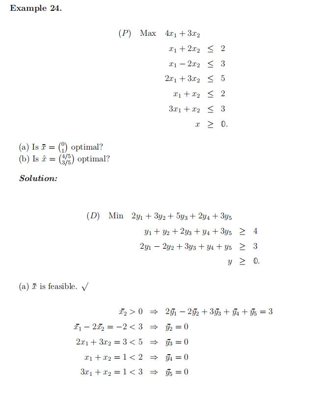
Example 11. Consider
(P ) max z(x) := 2x1 +x2
x1 −2x2 ≤ 2 4x1 +2x2 ≤ 10
−x1 ≤ 0
−x2 ≤ 0.
Consider x∗ = Σx∗1Σ := Σ 0 Σ is clearly a feasible solution.
Its objective value is Σ2 1Σ · Σ 0 Σ = 10.
Claim 1. x∗ is an optimal solution.
Consider the matrix representation of constraints of P :
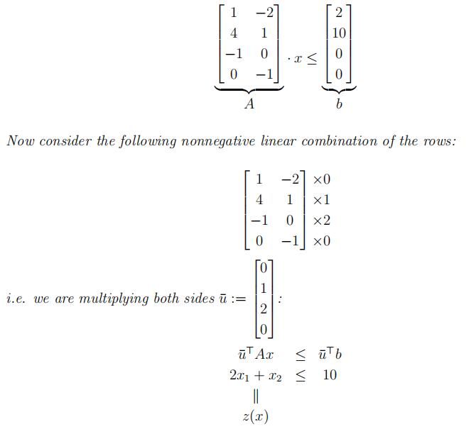
Note: This is a consequence of previous inequalities, i.e., ∀x such that Ax ≤ b ⇒ u¯TAx ≤u¯Tb. (Note that converse doesn’t necessarily hold.)
Here, we proved that ∀x ∈ R2 which satisfies all the constraints also satisfy:
z(x) = 2x1 + x2 ≤ 10.
Moreover, x∗ achieves the objective function value of 10.
⇒ x∗ is indeed optimal!
Remark 12. (1) In other words, for x ∈ Rn, if z(x) > 10, then x is not a feasible solution of the above LP.
(2) In fact, we will show that we can do this for all LP problems which have optimal solutions!
Now we give a graphical representation of this example in Fig. 1.
A few notes on this example:
- The shaded area is called feasible region which is the set of all feasible
- Optimal solution is attained at an extreme point of the feasible region. (We will provethis is always the case for LP s in either standard )
- Theobjective function vector is a non-negative linear combination of the constraint vectors. (We will prove this, )
- In this case, x∗is the unique optimal solution. However, in general, optimal solution may not be A small modification of our example can result in infinitely many optimal solutions. For example, let z := 0 or z := 4x1 + x2 instead.
An LP problem is unbounded if for every M ∈ R, there exists a feasible solution of the LP whose objective value is better than M .
Given a set S ⊆ Rn, we say that S is bounded if there exists a positive real number M
such that
S ⊆ {x ∈ Rn : −M 1 ≤ x ≤ M 1} .
If no such M exists, we say that the set S is unbounded. Note that an LP problem being unbounded is not equivalent to the statement that the feasible region of the LP problem is unbounded. In fact, some LP problems may have optimal solution(s) even if their feasible regions are unbounded.
In general, an LP problem can:
- have an optimal solution orsolutions,
- beinfeasible,
- beunbounded,
and these are the three only possibilities.
3.1Weak Duality Relation.
Let A ∈ Rm×n, b ∈ Rm, c ∈ Rn be Consider,
Max cTx
s.t. Ax ≤ b,
x ≥ 0.
We call this the primal problem (P ).
Then we define its dual problem (D), based on the same data (A, b, c):
Min bTy
s.t. ATy ≥ c,
x ≥ 0.
Then we have
Theorem 13.OPTIMIZATION代写
(Weak Duality Relation) For every feasible solution x¯ feasible solution y¯ of (D), we have of (P ) and every
cTx¯ ≤ bTy¯.
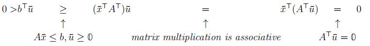
Proof. Suppose x¯ and y¯ are feasible solutions of (P ) and (D) respectively. Then
cTx¯ ≤ (ATy¯)Tx¯ = y¯T(Ax¯) ≤ y¯Tb = bTy¯,
where the first inequality follows from ATy¯ ≥ c, x¯ ≥ 0; the first equation follows frommatrix transposition and the associativity of matrix multiplication; the second inequalityfollows from Ax¯ ≤ b, y¯ ≥ 0; finally, the last equation is just the transpose of a scalar being equal to itself.
Corollary 14.
If x¯ and y¯ are feasible solutions of (P ) and (D) respectively and
cTx¯ = bTy¯
then x¯ is optimal in (P ) and y¯ is optimal in (D).
Proof. Forevery feasible solution x of (P ), by the last theorem, we have
cTx ≤ bTy¯ = cTx¯.
Thus, by definition (of an optimal solution), x¯ is an optimal solution of (P ).
Similarly, for every feasible solution y of (D), by the last theorem, we have
bTy ≥ cTx¯ = bTy¯.
Thus, by definition (of an optimal solution), y¯ is an optimal solution of (D).
Corollary 15. If (P ) is unbounded, then (D) is infeasible. If (D) is unbounded, then (P )is infeasible.
Proof. Assume (D) has a feasible solution y¯. Then, by the Weak Duality Relation, cTx ≤bTy¯, for every feasible solution x of (P ). Therefore, (P ) cannot be unbounded.
Similarly, assume (P ) has a feasible solution x¯. Then, by the Weak Duality Relation,bTy ≥ cTx¯, for every feasible solution y of (D). Therefore, (D) cannot be unbounded. Q
3.2. Strong Duality Theorems.OPTIMIZATION代写
Theorem 16. (A Strong Duality Theorem) Suppose both (P ) and (D) have feasible so- lutions. Then, they both have optimal solutions x∗, y∗. Moreover,
cTx∗ = bTy∗.
Proof. Suppose x¯ and y¯ are feasible solutions of (P ) and (D) respectively. Then consider
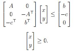
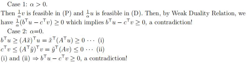
If this system has a solution, then by a corollary of the Weak Duality Relation, that is Corollary 14, we have x˜, y˜ feasible in (P) and (D) with cTx˜ = bTy˜, and hence, we are done.
We may assume the system has no solution.
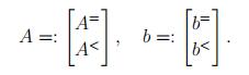
By the Theorem of the Alternative, there exist u ∈ Rm. v ∈ Rn , α ∈ R+ such that:
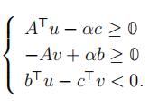
Focus on α.
Lemma 17. If (P) is feasible and (D) is infeasible, then (P) is unbounded.
Proof. Suppose x˜ is a feasible solution of (P) and (D) is infeasible. Then ATy ≥ c
y ≥ 0has no solution. By the Theorem of the Alternative, ∃d ∈ Rn, d ≥ 0, −Ad ≥ 0, −cTd < 0. Equivalently, Ad ≤ 0, d ≥ 0, cTd > 0.
Consider x(λ) := x˜ + λd, where λ ∈ R+. For every λ ∈ R+, x(λ) is a feasible solution of
(P):
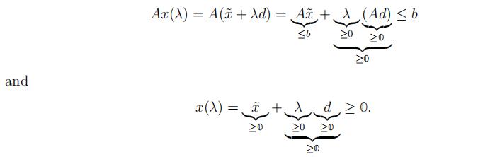
Moreover, the objective function value:
≥˛¸0cTx(λ) = cT(x˜ + λd) = cTx˜ + λ(cTd) → +∞, as λ → +∞. Therefore, (P) is unbounded.
Theorem 18.
(A Strong Duality Theorem) If (P) has an optimal solution, then so does (D) and their optimal objective values are the same.
Proof. Since (P) has feasible solution(s), if (D) also has feasible solution(s), then we are done by the previous theorem. If (D) has no solutions, then (D) is infeasible and by the previous lemma we reach a contradiction.
Theorem 19. (Fundamental Theorem of LP) Every LP problem has one of the following properties:
(I)LP has optimalsolution(s);
(II)LP isunbounded;
(III)LP isinfeasible.
Proof. (P) is either feasible or infeasible. If (P) is infeasible, then it satisfies (III).
if (P) is feasible and (D) is infeasible, then by the last lemma, (P) is unbounded. So it satisfies (II).
if (P) is feasible and (D) is feasible, then by The Strong Duality Theorem, (P) has optimal solution(s). So it satisfies (I).
Note that the dual of the dual of an LP problem is equivalent to the primal problem itself. Possibilities for (P) and (D)
| (P) \ (D) | has optimal solution(s) | unbounded | infeasible |
| has optimal solution(s) | √ | X | X |
| unbounded | X | X | √ |
| infeasible | X | √ | √ |
In the above, “X” means “impossible,” “√” means “possible.” As a by-product of our work so far,
we proved:
Proposition 20. For every A ∈ Rm×n, b ∈ Rm and c ∈ Rn, the set of primal-dual optimal solution pairs is:
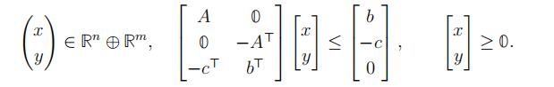
This result also indicates that solving LP problems is equivalent to solving systems of linear inequalities.
3.3ComplementarySlackness Conditions andTheorems.
Let’s look at the proofof Weak Duality Relation from the point of view of characterizing optimality.
For every feasible x¯ in (P ), ∀ feasible y¯ in (D), we have:
cTx¯ ≤ (ATy¯)Tx¯ = y¯T(Ax¯) ≤ y¯Tb.
Then x¯ is optimal in (P ), y¯ is optimal in (D), if and only if:
cTx¯ = (ATy¯)Tx¯ = y¯T(Ax¯) = y¯Tb.
Thus, x¯,y¯ are optimal in their respective problems if and only if:
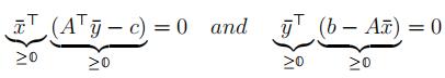
Definition 21. Complementary Slackness (CS) conditions:
∀j ∈ {1, 2, . . . , n}, either x¯j = 0 or (ATy¯ − c)j = 0, possibly both; and ∀i ∈ {1, 2, . . . , m}, either y¯i = 0 or (b − Ax¯)i = 0, possibly both.
Theorem 22. Let x¯ be feasible in (P ), y¯ be feasible in (D). Then x¯ and y¯ are optimal in (P ) and (D) respectively, if and only if they satisfy C.S. conditions.
Theorem 23. (Complementary Slackness Conditions) Let x¯ ∈ Rn then x¯ is optimal in
(P ) if and only if:
(I)x¯is feasible in (P )
(II)∃y¯∈ Rm, such that y¯ is feasible in (D) and satisfies S. conditions for x¯

y¯ is feasible in (D). Therefore, xˆ is optimal in (P ) and y¯ is optimal in (D).
Even though the above theorem can be very useful in many cases, in others, it may be useless. For example, given A ∈ Rm×n, c ∈ Rn, consider the following problem called (P ):
Max cTx
s.t. Ax ≤ 0
x ≥ 0.
Is x¯ := 0 optimal for (P )?
x¯ is at least feasible in (P). Let’s look at the dual problem (D).
Min 0Ty
s.t. ATy ≥ c
y ≥ 0.
However,
- Ax¯= 0 ⇒ Nothing about y from Complementary Slackness.
- x¯= 0 ⇒ Nothing about y from Complementary Slackness.
- ∴x¯ is optimal in (P ) iff (D) has a feasible Slackness.
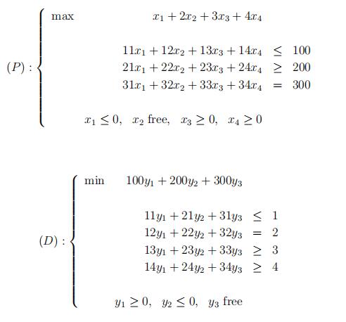
3.4Dualsof LP Problems in General Forms.
Every LP problem can be put into standard inequality from and we defined the dual for the latter, therefore we implicitly defined duals of all LP problems. Now, we make this more concrete.
3.4.1.Transformations.
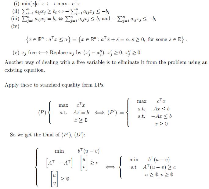
With y := u − v, we get
min bTy
s.t. ATy ≥ c
y free.
3.5General Recipe for the Dual Problem.
Where the Primal Problem has objec- tive function ”max …”, the Dual has objective function ”min…”.
| Primal | Dual |
| i’th constraint is ”≤” type i’th constraint is ”≥” type i’th constraint is ”=” type | i’th variable is restricted to ”≥ 0” i’th variable is restricted to ”≤ 0” i’th variable is free |
| j’th variable is restricted to ”≥ 0” j’th variable is restricted to ”≤ 0” j’th variable is free | j’th constraint is ”≥” type j’th constraint is ”≤” type j’th constraint is ”=” type |
We can take this table as the rigorous definition of the dual of an LP problem. Re- call that the dual of the dual of an LP problem is equivalent to the primal problem itself.
Example (for using the general recipe):
Summary of Theorems for LPs in an Arbitrary Form
Theorem 25. (Strong Duality Theorem for general form LPs) Let (P) and (D) be a pair of primal dual LP problems. Then,
(a)If (P) and (D) both have feasible solutions, then they both have optimal solutions and their optimal objective values are the
(b)If one of (P),(D) has an optimal solution, so does the other and their optimal objective values are the same.
Theorem 26.
(CS Theorem for general LPs) Let (P), (D) be a pair of primal-dual LP problems and letx¯,y¯ be a feasible solutions for (P) and (D) respectively. Then,x¯ is optimal in (P) and y¯ is optimal in (D) iff
(a)∀j, either x¯j = 0 or y¯ satisfies the jth dual constaint with equality and
(b)∀i, either y¯i = 0 or x¯ satisfies the ith primal constraint with equality.
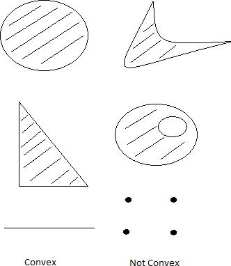
4.Polyhedra and ElementaryConvex Geometry
Figure Examples of convex sets and nonconvex sets in R2
Definition 27.
A set S ⊆ Rn is convex if ∀ u, v ∈ S and ∀ λ ∈ [0, 1], [λu + (1 − λ)v] ∈ S i.e, for every pair of points in the set, the line segment joining the pair lies entirely in the set.
It can be seen that if λ is chosen to be 1 then the resulting point will be u and if λ is chosen to be 0 then the resulting point will be v. Any other value of λ will result in a point between u, v. If λ is chosen to be 0.5 then it will result in a point exactly halfway between u, v.OPTIMIZATION代写
Some examples of convex sets are:
- Empty set,∅
- Closed unit ball {x ∈ Rn : ||x||2≤ 1}
- Open unit ball {x ∈ Rn : ||x||2< 1}
- Ellipsoids
- Linearsubspaces
- Halfspaces
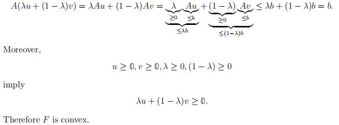
Example 28. Let A ∈ Rm×n, b ∈ Rm. Is F := {x ∈ Rn : Ax ≤ b, x ≥ 0} convex?
Let u, v ∈ F then,
u ≥ 0, v ≥ 0, Au ≤ b and Av ≤ b.
Let λ ∈ [0, 1] consider the vector,
[λu + (1 − λ)v] .Then,
Proposition 29. Intersection of any family of convex sets is convex.
Definition 30. S ⊆ Rn is a polyhedron if it is the intersection of finitely many closed half-spaces.
Closed half-space is defined as: {x ∈ Rn : aTx ≤ α} for some a ∈ Rn, α ∈ R.
Remark 31.OPTIMIZATION代写
(1)Feasible regions of LPs are convex.
(2)The set of optimal solutions of LPs are convex.
Let S ⊆ Rn. Then the convex hull of S is the intersection of all convex sets containingS. We denote it by conv(S).Given x(1), x(2), . . . , x(k) ∈ Rn, then Σk λjx(j) is called a convex combination of x(1), x(2), . . . , x(k) if λ ≥ 0 and 1Tλ = 1.
Proposition 32. S ⊆ Rn is a convex set iff it contains all convex combinations of its points.
Note that the above result provides an ”internal” definition for convex hulls.
Proof. (⇐=) Since S contains all convex combinations of its elements, it suffices to apply to every pair of elements, establishing the convexity of S.
(=⇒) We will proceed by induction on the number of points in a convex combination.
k = 1 is trivial.OPTIMIZATION代写
k = 2 follows from the definition of convex set.
Suppose the claim holds for all k ≤ A.
Let x(1), …, x(A+1) ∈ S, let λ ∈ RA+1, 1Tλ = 1. We may assume λ > 0. Then,
Therefore, xˆ is a convex combination of x(1), . . . , x(A) and by the induction hypothesis,xˆ ∈ S.
By (∗) and the assumption that S is convex (since xˆ, x(A+1) ∈ S and λA+1 ∈ (0, 1)),A+1 (i)i=1
Corollary 33. For every S ⊆ Rn, the convex hull of S is the set of all convex combinations of elements of S.
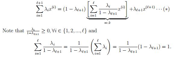
Theorem 34. (Carath´eodory [1907]) Let S ⊆ Rn. Then every point in conv(S) can be expressed as a convex combination of (n + 1) or fewer points in S.
Proof. Let x¯ ∈ conv(S) and x(1), …, x(k) ∈ S such that x¯
k i=1λix(i), where λ ∈Rn , 1Tλ = 1.
We may assume k ≥ n + 2 and λ > 0.
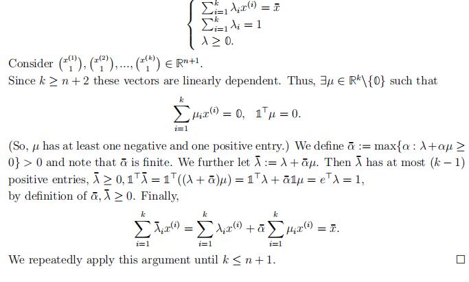
In the above proof, we used the observation that the vectors .x(1)Σ, .x(2)Σ, . . . , .x(k)Σ ∈Rn+1 are linearly dependent (since k n + 2). This leads us to a definition:
A set of vectors .x(1), . . . , x(k)Σ ⊂ Rn is affinely independent if
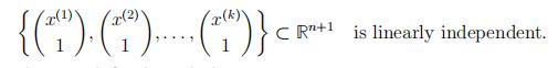
Affine dependence is defined similarly.OPTIMIZATION代写
Note that x(1), . . . , x(k) ⊂ Rn is affinely independent iff
x(2) − x(1), x(3) − x(1), . . . , x(k) − x(1) ⊂ Rn is linearly independent.
In this statement, choice of x(1) is arbitrary (any x(i) in its place would do). This equiva- lent definition highlights the fact that the notions of affine independence/dependence are invariant under translation of the set by any point in Rn. Note that the same is not true for the notions of linear dependence/independence.
4.1. Extreme Points of Convex Sets, Internal Structure of Polyhedra.
Let S ⊆ Rn be a convex set. Then,
x¯ = 1 u + 1 v.x¯ ∈ S is an extreme point of S if $u, v ∈ S\{x¯} such that
Theorem 35. Let S ⊆ Rn be a convex set. Then x¯ ∈ S is an extreme point of S iff S\{x¯}is convex.
Given x¯ ∈ Rn such that Ax¯ ≤ b, denote by A= is the matrix formed by the rows of A for which x¯ satisfies x satisfifies (Ax)i ≤ bi with equality.
Theorem 36.
Let A ∈ Rm×n, b ∈ Rm, F := {x ∈ Rn : Ax ≤ b}, x¯ ∈ F . Also let{A=x ≤ b=} denote the subset of inequalities in {Ax ≤ b} satisfied as equality by
Then, x¯ is an extreme point of F iff rank(A=) = n.OPTIMIZATION代写
Proof. (⇒): Suppose rank(A=) ƒ= n. Then rank(A=) < n.x¯.
Thus, ∃ a linear dependence d ∈ Rn\{0} among the columns of A= such that A=d = 0. There exists ε > 0, small enough such that A<(x¯ ± εd) ≤ b<,
Moreover, A=(x ± εd) = A=x ±ε A=d = b=.
![]()
Therefore, x¯ is not an extreme point of F .OPTIMIZATION代写
We will use the following lemma for the remaining part of the proof.
Lemma 36.
(a) Let a, x¯ ∈ Rn, α ∈ R such that aTx¯ = α. Then for every x(1), x(2) ∈ Rn, such that aTx(1) ≤ α, aTx(2) ≤ α, x¯ = 1 x(1) + 1 x(2), we have aTx(1) = aTx(1) = α.
Proof. Let a,x¯, x(1), x(2), α be as above. Then,
α ≥ 1 aTx(1) + 1 aTx(2) = aT Σ 1 x(1) + 1 x(2)Σ = aTx¯ = α.
Since aTx(1) ≤ α, aTx(2) ≤ α, we have aTx(1) = aTx(1) = α. Q
Proof of the theorem continued:
(⇐): Suppose rank(A=) = n. Further suppose x¯ is not an extreme point of F . (We are seeking a contradiction.)
Then, ∃ x(1), x(2) ∈ F \{x} such that x¯ = 1 x(1) + 1 x(2).OPTIMIZATION代写
By the last lemma, A=x(1) = A=x(2) = b=.
However, rank(A=) = n, which implies A=x = b= has a unique solution, we have three distinct solutions x, x(1), x(2), a contradiction. Q
Corollary 37.
(I)Ifrank(A) < n, then F has no extreme
(II)Thenumber of extreme points of every polyhedron is
(E.g., in the above case, m is an upper bound on the number of extreme points.)
Definition 38. A polyhedron in Rn is called pointed if it does not contain any lines.
Note that every polyhedron of the form {x ∈ Rn : Ax ≤ b, x ≥ 0} is pointed. So is
{x ∈ Rn : Ax = b, x ≥ 0}.OPTIMIZATION代写
Recall, every line in Rn can be expressed as {λx(1) + (1 − λ)x(2) : λ ∈ R} for some pair of points x(1), x(2) ∈ Rn.
Proposition 39. Suppose P ⊆ Rn is a nonempty polyhedron. Then, P is pointed iff P has at least one extreme point.OPTIMIZATION代写
Theorem 40. If an LP problem has an optimal solution and its feasible region is pointed (i.e. it contains no lines) then the LP problem has an optimal solution which is an extreme point of the feasible region.
Proof. We may assume that our LP is in the form:
Max cTx
s.t. x ∈ F where F := {x ∈ Rn : Ax ≤ b}.
Pick an optimal solution x¯ of the LP such that x¯ satisfies as many inequalities of {Ax ≤ b} as possible with equality. We claim that x¯ is an extreme point of F .
Assume not (we are seeking a contradiction). Then ∃x(1), x(2) ∈ F \{x¯} such thatx¯ x(1)+ x(2) . By Lemma 36(a), cTx¯= cTx(1) = cTx(2). Also by this lemma, since
A=x¯ = b=, x(1) and x(2) also satisfy the same equations with equality – that is, they both satisfy A=x = b=.
Now consider the line L going through x(1) and x(2),
that is L := {λx(1) + (1 − λ)x(2) : λ ∈ R}. Recall that x¯ ∈ L. Expanding on the same arguments used before, we observethat every point x ∈ L satisfies cTx = cTx¯ and A=x = b=. Since F contains no lines,there is a maximum or minimum value of λ for which λx(1) + (1 − λ)x(2) ∈ F : call it λ¯.Then xj = λ¯x(1) + (1 − λ¯)x(2) is optimal, but it satisfies at least one more inequality fromA<x ≤ b< with equality, a contradiction. Thus x¯ is an extreme point, and the proof is complete.OPTIMIZATION代写
Remark 41.This theorem provides an algebraic characterization of a fundamental, geo- metric object (as we will crystalize in the upcoming theorems). Moreover, it indicates, among other things, a finite (though very silly and inefficient) algorithm to solve LPs; every LP can be solved by putting it into one of the stated forms and enumerating all the extreme points of the feasible region of the reformulation. However, this algorithm does not address detecting unboundedness of the LP at hand (this can be addressed by considering extreme rays of F and obtaining a similar algebraic characterization of them).
4.2. Polytopes.
Definition 42. A bounded polyhedron is called a polytope. Bounded polyhedra are called polytopes.
Note that polytopes are compact (closed & bounded).
Theorem 43. Let F ⊂ Rn be a polytope. Then, F is equal to the convex hull of its extreme points.
Proof. We may assume F ƒ= ∅. Let {v1), . . . , v(k)} be the extreme points of F (there is at least one, and there are finitely many by Theorem 36). Let F¯ denote the convex hullof F , i.e. F¯ := conv{v(1), …, v(k)}. By definition of convex hull and convexity of F , F¯ ⊆ F .OPTIMIZATION代写
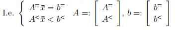
Assume for a contradiction that the other containment is not true, i.e., ∃x¯ ∈ F \F¯. Now consider the system:
kj=1 kλjv(j) = x¯λj = 1
j=1
λ ≥ 0.
This system has no solution due to the internal characterization of convex hulls. By a theorem of the alternative (specifically, Farkas’ Lemma), ∃µ ∈ Rn, η ∈ R such that
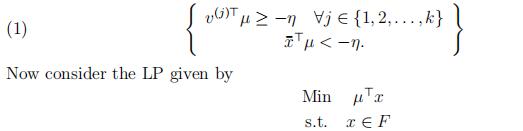
Since F is a polytope, F contains no lines and since it is nonempty and bounded, by the Fundamental Theorem of LPs, this LP has an optimal solution(s). By the last theorem,there is an optimal solution that is also an extreme point of F . However, the condition (1) implies that none of the extreme points of F is optimal, which is a contradiction. Thus,
F = F¯. Q
It is also true that:
Theorem 44. Convex hull of any finite set in Rn is a polytope.
For any pair of sets S1, S2 ⊆ Rn, the Minkowski sum of S1 and S2 is defined by
S1 + S2 := {u + v : u ∈ S1, v ∈ S2} .
K ⊆ Rn is a polyhedral cone if it is a polyhedron and it is a cone. In particular, every nonempty polyhedral cone in Rn can be expressed as
K = {x ∈ Rn : Ax ≤ 0}
for some A ∈ Rm×n, for some positive integer m.OPTIMIZATION代写
Theorem 45. Let F ⊂ Rn be a nonempty pointed polyhedron. Then, there exists a polytope P ⊂ Rn and a pointed polyhedral cone K ⊂ Rn such that
F = P + K.
The above decomposition of F is not unique in general. However, let ext(F ) denote the set of extreme points of of F . Then, we can have a unique decomposition of such F , with P := ext(F ).
S ⊆ Rn is an affine subspace if there exist, an integer m, A ∈ Rm×n and b ∈ Rm such that
S = {x ∈ Rn : Ax = b} .
Theorem 46. Let F ⊂ Rn be a nonempty polyhedron. Then, there exists a polytope
P ⊂ Rn, a pointed polyhedral cone K ⊂ Rn, and an affine subspace L ⊆ Rn such that
F = P + K + L,
where L is the lineality space of F .OPTIMIZATION代写
Similar to the comment we made following Theorem 45, we can take P := ext(F ) in the above theorem.
Related to above characterizations of polytopes, there is a generalization to infinite- dimensional spaces (known as the Krein-Milman Theorem). Below, we state a version of it for Euclidean spaces (definitions of some of the terms below will be covered later in the course, e.g., cl(·) denotes the closure of a set):
Let C ⊂ Rn be a compact convex set, and let S ⊆ C. Then, the following are equivalent:
(i)cl (conv(S)) =C;
(ii)inf hTx : x∈ S = min hTx : x ∈ C ;
(iii)ext(C) ⊆cl(S).
5.SimplexMethod
We will explain after designing the algorithms the name “Simplex Method.” However, first let’s cover what the word simplex means in this context.
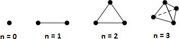
A simplex in Rn is the convex hull of (n+1) affinely independent points υ(1), υ(2), …, υ(n+1) ∈Rn.
Points υ(1), υ(2), …, υ(k) ∈ Rn are affinely independent if
Rn+1 are linearly independent. Simplicies in Rn:
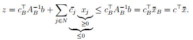
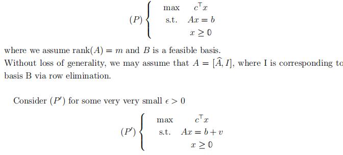
We will work with LPs in standard equality form:
(P ) Max cTx
s.t. Ax = b,
x ≥ 0.
where A ∈ Rm×n, b ∈ Rm, and c ∈ Rn.
Wlog, we may assume rank(A) = m. If not, apply row reduction to [ A|b ] either proving that Ax = b has no solution ((P) is infeasible) or finding redundant equations and then
eliminating these redundant equations from Ax = b.
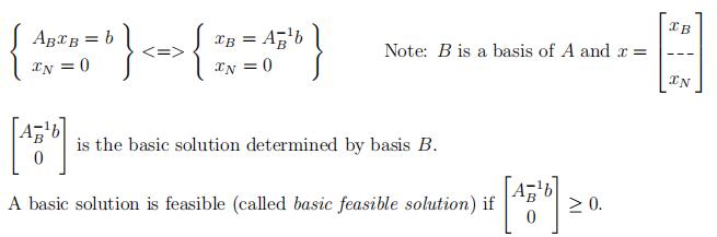
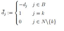
Given B ⊆ {1, 2, …, n}, we define N = {1, 2, …, n}\B. We write:
A := [A1 A2··An]
B and N give a partition of the columns of A:
AB := [Ai : i ∈ B]
AN := [Aj : j ∈ N ]
A subset B ⊆ {1, 2, …, n} is called a basis of A if |B| = m and AB is non-singular (i.e. invertible).OPTIMIZATION代写
A basic solution of Ax = b is the unique solution of Ax = b .xN = 0
Theorem 47. Let A ∈ Rm×n, b ∈ Rm such that rank(A) = m. Further let
F := {x ∈ Rn : Ax = b, x ≥ 0}
and suppose x¯ ∈ F . Then, the following are equivalent:
(i)x¯is a basic feasible solution of Ax = b ;x ≥ 0
(ii){Aj: x¯j > 0} is linearly independent;
(iii)x¯is an extreme point of F .
Moreover, x¯ is a basic feasible solution of Ax = b x ≥ 0 iff x¯ is an extreme point of F .
Suppose we are working with an LP problem in standard equality form:
(P ) : Max z = cTx
s.t. Ax = b, x ≥ 0,
where A is an m-by-n matrix of rank m.OPTIMIZATION代写
Denote A = A1 ….. An , where Ai represents the columns of the matrix A. Let
B ⊆ {1, 2, …, n} be a basis for A and N = {1, 2, …, n}\B, then, we have
Definition 48. feasible basis B of (P ):
A basis B of A such that the basic solution determined by B is a basic feasible solution of {Ax = b, x ≥ 0}.
Suppose further that we set xN := 0, then the system
(*) Ax = b ⇐⇒ ABxB + AN xN = b
uniquely identifies the current basic feasible solution
(since A−1 is non-singular).
x¯ =
x¯B = B
x¯N 0
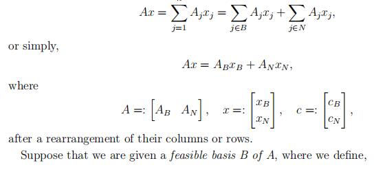
So, how do we change our current solution to improve the objective value z? Since we
have set xN = 0, if we want to consider other feasible solutions of (*), we have to pick at least one j ∈ N and set xj to some nonzero value.OPTIMIZATION代写
Assume k ∈ N is the one we pick. To maintain feasibility of the new solution, we must set
xk := α ≥ 0.
Moreover, to maintain Ax = b, by the relation
ABxB + Akxk = b,
(Note that the LP problem (P ) may not be unbounded.) If the above case does not occur,x¯new is our new basic feasible solution.OPTIMIZATION代写
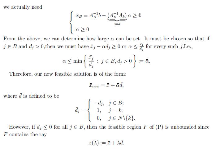
How can we be sure that the k ∈ N that we’ve picked actually did improve the objective value z? Let’s take a look at z:
z = cTx = cTB xB + cTN xN ,
by (*), we see that for all basic feasible solutions xB,
z = cTB A−1b − (A−1AN xN ) + cTN xN
= cTB A−1b + (cTN − cTB A−1AN )xN
Let y¯ be the unique solution to the system: ATB y = cB, then,
z = cTB A−1b
= objective valuse of˛t¸he cxurrent solution x¯
+(cTN − y¯TAN )xN
= constant + Σj∈N c¯jxj,
where c¯j, j ∈ N are the entries of the vector c¯N := cTN − y¯TAN and is called the reduced cost of xj with respect to the current basis B.OPTIMIZATION代写
From the above, we see that c¯k behaves like the partial derivative of the objective function with respect to xk: c¯k ≈and in order to improve our current solution, we need to choose a k ∈ N such that c¯j ≤ 0 ∀j ∈ N .
Claim. If the inequality
c¯k > 0.
holds (based on the current index sets B, N), then the current solution x¯ is an optimal solution for (P).
We provide two proofs here.
Proof. (1)
For all feasible solutions x, recall that
The above proves that the current basic feasible solution x¯ is optimal for (P ). The abovearguments can be adopted to prove that if c¯j < 0 for every j ∈ N , then the current basicfeasible solution x¯ is the unique optimal solution of (P ). To see this, notice that for everyfeasible solution of (P ) except x¯, we must have xj > 0 for some j ∈ N . Since c¯j < 0 for every j ∈ N , this implies that for every feasible solution of (P ) except x¯, we have
z < cTx¯.OPTIMIZATION代写
Therefore, x¯ is the unique optimal solution of (P ) in this case.
Proof. (2)
Consider the dual problem of (P):
(D) : Min bTy
s.t. ATy ≥ c,
y free.
Since ATB y¯ = cB, and by the assumption cTN − y¯TAN ≤ 0T, we immediately see that y¯ is a feasible solution of (D). Let’s check if it is an optimal solution. Indeed,
bTy¯ = bT(A−TcB) = cTB A−1b = cTx¯.
Hence, by the corresponding corollary of the Weak Duality Theorem, x¯ is an optimal solution for (P) and y¯ is an optimal solution of (D).
where A ∈ Rm×n, rank(A) = m.
Simplex Method OPTIMIZATION代写
Input A, b, c for an LP in SEF, a basic feasible solution x¯ determined by a basis B ofA.(A, b, c, x¯, B), N := {1, 2, …, n}\{B}.
(1)SolveATB y = cB.
(2)Computec¯j := cj − yTAj, ∀j ∈ N .
Ifc¯j ≤ 0, ∀j ∈ N then STOP
x¯ is an optimal solution of (P), y is an optimal solution of (D) else pick k ∈ N such that c¯k > 0.OPTIMIZATION代写
(4)Solve ABd =Ak,
(5)If d ≤ 0 (or, equivalently d¯ ≥ 0) thenSTOP
(P) is unbounded (proof: x¯, d¯)
x(λ) := x¯ + λd feasible in (P), ∀λ ≥ 0 and cTx(λ) = cTx + λc¯k → +∞ as λ → +∞
(D) is infeasible (proof: d¯)
d¯ satisfies: d¯ ≥ 0, Ad¯ = 0, cTd¯ = c¯k > 0
(6)Pick r ∈ B such that dr> 0 and
x¯r dr = min¯xi di : i ∈ B, di > 0 =: ¯α
(7) x¯ := x¯ + α¯d¯
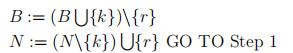
Steps (3) and (6) only mention eligibility rules for entering and leaving indices (k and r). They do not uniquely specify these choices. To make steps (3) and (6) well-defined, consider for example, the Smallest Subscript Rule (also known as Bland’s Rule).
Among all j ∈ N such that c¯j > 0 pick k := min{j ∈ N : c¯j > 0}.
Among all A ∈ B such that dA > 0 and
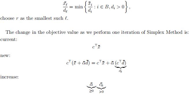
Theorem 49. If Simplex Method applied to an LP in SEF, with a starting basic feasible solution, never encounters α¯ = 0, then in at most .n Σ iterations it terminates, either providing optimal solutions for (P) and (D), or a proof that (P) is unbounded and (D) is infeasible.OPTIMIZATION代写
Proof. There are at most n feasible bases and since α¯c¯k > 0, in every iteration, no basis will be repeated.
Definition 50. A basic solution x¯ for Ax = b, determined by a basis B of A is called degenerate if for some i ∈ B, x¯i = 0. Otherwise, x¯ is a nondegenerate basic solution.
We similarly define degenerate basis, degenerate basic feasible solution.
Definition 51. (P) is called nondegenerate if every basis B of A is nondegenerate.
Theorem 52. Simplex Method applied to an LP in SEF, with a starting basic feasible solution, and using the smallest subscript rule (Bland’s Rule), terminates in at most .n Σ iterations.
Proof. Proof will be provided later, as part of Assignment 3.
Suppose we are using well-defined deterministic rules for the choice of k and r so that the rules are consistent under given basis B, which means if the algorithm picks k and r when B is the current bases, the next time algorithm encounters B as the current basis, it again chooses k and r.
If such implementation of the simplex method dose not terminate, then it must cycle.
For example,the sequence of feasible bases: B0, B1, . . . , Bl, . . . , Bl+q, Bl, Bl+1, . . .
s a ˛cy¸cle x
leads to cycling. Note that all basic feasible solutions in the cycle here are degenerate, which means that the objective value as well as the basic feasible solution x¯ remains the same.
Hoffman [1953] was the first to construct an example and prove that Simplex Method can cycle. Of course, smallest subscript rules prevent cycling. We will see another, far- reaching idea to remedy the situation next.
5.1.Lexicographic simplex method.
This result goes back to 1951. The mainidea
goes much farther back. Let A ∈ Rm×n, b ∈ Rm, c ∈ Rn be given. Consider,
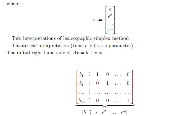
Note that we can view b as the most significant digit and sm as the least significant digit.
When we apply simplex method to (P j), we can compare xiilexicographically.
For a basis B of (P ), we have
XB := hAB1b … AB1iin (P j)
in (P0)
Note that even when (P) is degenerate, which means there exists zero entry of A−1b, XBdoes not have a zero entry, since this would mean, it has a whole row of zeroes which is impossible as A−1B is nonsingular. Therefore, (P j) is nondegenerate. Note that this approach induces a strict order among the feasible bases of B.
We have proved the following proposition.OPTIMIZATION代写
Proposition 53. The LP problem (P j) is nondegenerate.
Practical Interpretation: Choose a very small value of s and perturb the right hand side b explicitly, say by randomly chosen positive values for each i, with mean s), then later in the computation, when it is safe, remove the perturbation.
In practice the danger is not cycling but stalling (going through a very long sequence of degenerate solutions without changing x)
Theorem 54. Lexicographic Simplex Method applied to (P’) terminates in at most n iterations. If it terminates proving (P’) is unbounded then this leads to a proof that (P) is unbounded; If it terminates with an optimal basis B for (P’) then B is an optimal basis for (P).
i.e.Solving (P’) solves(P).
Summary:
Degeneracy can lead to:
(i)Cycling (but this turns out not to be a problem inpractice)
(ii)Stalling (this is a potential problem inpractice)OPTIMIZATION代写
Main Idea: Perturb the original problem. We can do this by modifying bi by a small amount, but different amounts for each bi
Remark: Non-degeneracy is generic in the sense that randomly generated LP’s are non-degenerate. One should note however that in practice LP’s are often formulated which are degenerate.
There are two interpretations of this.
1)Theoretical: Lexicographic Simplex Method (we can implement without mentionings’s)
2)Practical: We pick values fors.
e.g., si randomly distributed with mean 10−12 and an even smaller variance. (Note that this is not choosing increasing powers of s.)
At this point, we would be forgiven for being a bit skeptical of the Simplex Method. The method is certainly well-known and used widely in practice. We have heard that the method is very efficient but at the present moment, we cannot use it. Remember, the Simplex Method takes us from one basic feasible solution to another. Given a basis B with basic feasible solution x¯, the Simplex Algorithm will choose a new basis Bj, withm − 1 indices from B and one new index from B’s complement N , and also compute thecorresponding basic feasible solution xˆ. That is all well and good, but we currently have no way of choosing an initial basis B and its corresponding basic feasible solution.OPTIMIZATION代写
Of course,
we do not want to check through all possible bases until we find a suitable starting point. That would potentially lead to checking all n bases, which would be inefficient and, if we did end up checking all bases, render the Simplex method pointless (as we would have seen all possible basic feasible solutions already, and so we would just pick the one with the largest objective value). This is clearly not the standard practice, so how can we efficiently choose a starting basis?
As it turns out, choosing a feasible basis can be reformulated as solving an auxiliary LP problem which has an obvious feasible basis. We can apply simplex method to the auxiliary LP problem to give us a basis B for the original LP problem, then use simplex algorithm on the original LP with B as our initial basis.
To see how this works,
let us start by solving another issue with simplex method. Cur- rently, our method requires an LP problem in standard equality form. Suppose we are given the following LP in standard inequality form.OPTIMIZATION代写
max cTx
s.t. Ax ≤ b x ≥ 0.
with b ≥ 0. Then we introduce slack variables xn+1, …, xn+m ≥ 0 and consider
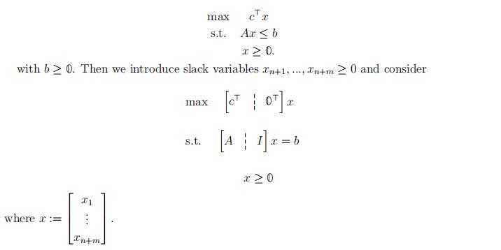
Note that in thisΣcase, BΣ= {n + 1, n + 2, . . . , n + m} is a feasible basis (we can see this (P ) max cTx s.t. Ax = b x ≥ 0,
but with no obvious starting basic feasible solution.
We may assume b ≥ 0 (since we can multiply rows by −1 if necessary).
Let’s introduce something we will call artificial variables xn+1, . . . , xn+m ≥ 0, (unlike when we introduced slack variables above, these artificial variables are not really a part of the problem) and consider the following auxiliary problem (Paux).
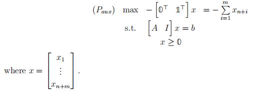
Remarks:
- B= {xn+1, . . . , xn+m} is a feasible basis for (Paux)OPTIMIZATION代写
- (Paux)has feasible solutions (see Remark 1). This LP is not The optimal
objective value is bounded above by zero. Recall that the objective function is equalto −Σmmi=1xn+i. All components of x are nonnegative so m i=1 xn+i is nonnegative, so always has an optimal solution(s).
- (P ) is infeasible iff the optimal objective value of (Paux) is negative. (If the optimal valueof (Paux) is negative, then the optimal solution has nonzero variables from{xn+1, . . . , xn+m}. A better solution would have all nonzero variables come from the original variables {x1, . . . , xn}. If such a solution cannot be found the original problem must be infeasible.)
This suggests the two phase method.OPTIMIZATION代写
Two Phase Method
0.Givenan LP (P ) in standard equality form, make sure rank(A) = m and b ≥ 0
1.Solve (Paux) using simplex
2.Ifthe optimal objective value of (Paux) is negative (P ) is infeasible, current y¯ is proof.
(Daux) min bTy
s.t. ATy ≥ 0
y ≥ −1
If y¯ is an optimal solution of (Daux) with bTy¯ < 0 then we have ATy¯ ≥ 0 and bTy¯ < 0 (by Farkas’ Lemma, (P ) is infeasible).
- We have a basic feasible solution of (Paux) with objective value Therefore,it
determines a basic feasible solution for (P ), say x¯.
- Solve(P ) starting with the basic feasible solution x¯ of (P ).
Note that some additional work may be necessary to find a basis B determining the basic feasible solution x¯ in Step 4 (between Phase I and Phase II).
Another Approach: Try to solve OPTIMIZATION代写
(P¯) max 0Tx (D¯ ) min bTy
s.t. Ax = b s.t. ATy ≥ 0
x ≥ 0
y¯ := 0 is a basic feasible solution to (D¯ ), so we can apply simplex method to (D¯ ) starting with the basic feasible solution y¯. At the end of solving (D¯ ) Simplex Method either proves that y¯ is an optimal solution of (D¯ ), or it proves that (D¯ ) is unbounded. In the lattercase, the proof of unboundedness of (D¯ ) leads to a proof of infeasibility of (P ) as before. The following is such an algorithm (i.e., an algorithm that applies the Simplex Method to the dual problem; from the point-of-view of the primal problem, it maintains dual feasibility and complementary slackness in every iteration, while striving to reach primal feasibility). Namely, Revised Dual Simplex Method : … OPTIMIZATION代写
The Simplex Interpretation of the Simplex Method (Dantzig) Suppose the given LP is in the form:
(P j) Max z := cTx
s.t. Ax = b 1¯Tx = 1 x ≥ 0
- Theform (P j) is general enough that if one has an algorithm to solve (P j) then that algorithm can be used as a black box, relatively efficiently to solve an arbitrary LP problem (P ).
- Thefeasible region of (P j) is bounded (it is a subset of the unit Simplex), therefore (P j) cannot be
- Thefeasible regions of (P j) and of the original problem (P ) are not necessarily equal.
The special form of (P j) allows us to interpret its feasible solutions as convex combina- tions of columns of A. In this interpretation, (P j) is feasible iff b is in the convex hull of columns Aj of A. This gives us a way of interpreting and representing solutions x (which are in Rn) in the column geometry given by A and b in Rm.
Therefore, including the objective function, we have a representation of (P j) in Rm+1 as depicted in the following figure.OPTIMIZATION代写
- The polygon in the above figure is not the feasible region of (P j); but it represents it. Every point in the intersection of the polygon with the line defined by [z, bT]Trepresents a feasible solution of (P j).
- Thedotted lines connecting points [ cj ATj ]T are m-dimensional simplices (they are convex hulls of (m + 1) points). Each such simplex corresponds to a basis. Note that in (P j), there are (m + 1) equations and a basis needs (m + 1) indices. Once a basis is picked, we have the (m + 1) corresponding points [cj, ATj ]T, for j ∈ B. If the convex hull of these (m + 1) points in Rm+1 intersect the line defined by [z, bT]T, then we have that the basis B defines a basic feasible solution.
- Thesepoints (corresponding to the Q points in the picture) represent feasible solutions, but they are not feasible solutions themselves.
- Inthe figure, the algorithm starts from the basic feasible solution determined by the basis B = {6, 7}. Here x6 and x7 are positive (and they add up to one) and
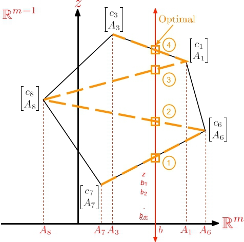
Figure 2. Geometric intuition behind the Simplex Algorithm.
all other xj’s are zero. In the first iteration, index 7 leaves the basis and index 8 enters the basis. The new basis is B = {6, 8} and it determines a basic feasible solution where x6 and x8 are positive (and they add up to one) and all other xj’s are zero. … Eventually, we arrive at the basis B = {1, 3} which determines the optimal solution where x1 and x3 are positive (and they add up to one) and all other xj’s are zero.
According to Dantzig, this is why he named the algorithm “Simplex Method”, and why he believed it would be efficient.OPTIMIZATION代写
5.2.Strict Complementarity Theorem.
We will conclude with a refinement of the Complementary Slackness Theorem.
Theorem 55 (Strict Complementarity Theorem). Suppose (P ) in standard equality form has optimal solution(s). Then (P ) and (D) have optimal solution x∗, y∗, such that for all j ∈ {1, 2, . . . , n}, we have x∗j (ATy∗ − c)j = 0 and x∗j + (ATy∗ − c)j > 0.
Proof. By the Strong Duality Theorem, both (P ) and (D) have optimal solutions with
the same objective value, say z∗. For each j ∈ {1, 2, . . . , n}, we will either construct
an optimal solution x(j) of (P ) with x(j) > 0, or an optimal solution y(j) of (D) with
(ATy(j) − c)j > 0. For each j, consider the primal-dual pair of LPs:
(Pj) Max xj
s.t. Ax = b
cTx ≥ z∗ x ≥ 0
(Dj) Min bTy + z∗η
s.t. ATy + ηc ≥ ej η ≤ 0.
The problem (Pj) has been formulated such that its feasible region is the set of optimal solutions of the original problem (P ). If (Pj) has feasible solution(s) with xj > 0, then we have an optimal solution x(j) of (P ), as desired. Otherwise, the optimal objective value of (Pj) is zero.OPTIMIZATION代写
By the Strong Duality Theorem, (Dj) has an optimal solution y¯, η¯ such that bTy¯ =−z∗η¯.
Case 1 η¯ = 0. Then ATy¯ ≥ ej, bTy¯ = 0. Take any optimal solution yˆ of (D), and let y(j) := yˆ + y¯. This y(j) satisfies constraint j with slack ≥ 1, and all others with slack ≥ 0.
Case 2 η¯ < 0. Take y(j) := y¯ . Then ATy(j) ≥ c − 1 ej, bTy(j) = bTy¯ = −z∗η¯ = z∗.
Let B denote the set of indices j for which we constructed x(j), and let N be its
complement. Then, by convexity of the optimal solution sets,
x∗ := 1 x(j)
|B| j∈B
y∗ := 1 y(j)
|N| j∈N
are desired optimal solutions. Note that one of B or N may be empty. If B = ∅, then
x∗ = 0. If N = ∅, then y∗ is the unique solution of ATy = c.OPTIMIZATION代写
6.Combinatorial Optimization OPTIMIZATION代写
Example 56. Assignment Problem
We have a set of jobs J and there is a set of workers W who can perform these jobs and we are given cij ∈ R, ∀i ∈ W, ∀j ∈ J representing compatibility of worker i and job j. The problem is to assign workers to jobs such that every worker gets one job and every job is assigned one worker and total compatibility of the assignment is maximized.
Let’s formulate as an optimization problem.
Such optimization problem, LPs + integrality constraints on a nonempty subset of vari- ables are called integer programming problems.OPTIMIZATION代写
Sometimes we make a distinction between two types of integer programming (IP) prob- lems.
- if all variables are required to be integers([pure] integer programmingproblems).
- if some variables are required to be integers and some are real-valued (mixed integerprogramming).OPTIMIZATION代写
The following is a MATLAB code that generates the LP formulation of the Assignment problem:
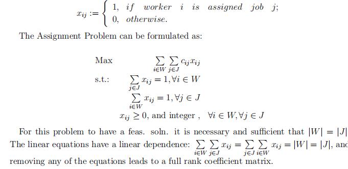
G = (V, E),
where G represents a graph, V is the set of nodes in the graphs, E is the set of edges in the graph. Edges are sets of pairs of nodes: e = {i, j} where e represents edge, i, j ∈ V .
V = {1, 2, 3, 4, 5}
E = {{1, 2}, {1, 5}, {2, 3}, {2, 5}, {3, 4}, {3, 5}, {4, 5}}
Such graphs are sometimes called undirected graphs, and sometimes simply graphs.
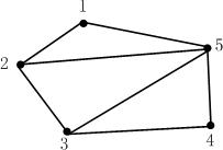
A graph is bipartite if there exists a partition [W, J] of V (i.e., W ∪J = V, W ∩J = ∅) such that all edges in E have one endpoint in W and the other in J.OPTIMIZATION代写
A matching in G is a subset of edges M such that every node in G is an endpoint of at most one edge in M . A perfect matching in G is a matching in G where |M | = |V | .
Given weights we, ∀e ∈ E, optimal matching problem is to find a matching M in G
e∈Msuch that we is maximized.
Assignment Problem is equivalent to optimal perfect matching problem on complete bipartite graphs.
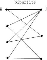
A directed graph (diagraph) is G˙ = (V, E˙) where the edges of the graph e ∈ E˙are directed (such edges are called arcs) and have the form (i, j).
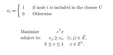
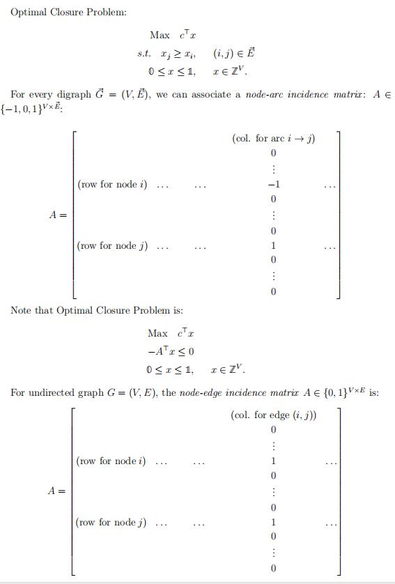
A subset C ⊆ V in~G = (V, ~E) is called closure if no arc in~G leaves C.
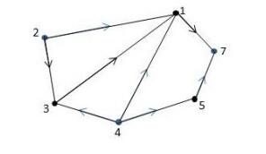
Note that the set V , and empty set are closures.OPTIMIZATION代写
Given weights Cv ∈ R for ∀v ∈ V ,the optimal closure problem is to find a closure C in G˙ such that cv is maximized.
A path (directed path, dipath) in a graph is a sequence OPTIMIZATION代写
v0e1v1e2v2…vk−1ekvk
where vi ∈ V and ei ∈ E(or ei ∈ E˙). Sometimes we use the term walk for a path.
A path is called simple if all v0, v1, …, vk are distinct. A path is a cycle if v0 = vk.
A cycle is a circuit if v0, v1, …vk−1 are distinct.
NOTE: Our graphs in this course will not have self-loops or parallel edges (arcs) unless explicitly specified. Further note that for directed graphs, arcs (i, j) and (j, i) are different, as a result, they are not considered parallel arcs in this context.
A simple path in G (or in G˙) is a Hamiltonian path if {v0, v1, …, vk} = V .
A circuit in G (or G˙)is a Hamiltonian cycle (or equivalently, Hamiltonian circuit) if {v0, v1, …, vk−1} = V .
Suppose we are given costs ce, ∀e ∈ E(or∀e ∈ E˙).OPTIMIZATION代写
Shortest path problem is to find a simple path from some node s ∈ V to some nodes t ∈ V of minimum cost.
For example, the costs can be the time needed to complete a task.
Longest path problem is to find a simple path from s ∈ V to t ∈ V of maximum cost. It can be used to find the bottleneck in completing a task(the costs are the times) or to determine which task consumes the most amount of resources.
NOTE: If the costs are ce ≥ 0∀e ∈ E(e ∈ E˙)and the shortest path problem is very easy, the longest path problem is NP-hard. If ce ≤ 0, the shortest path is the difficult one.Finding a Hamiltonian path or Hamiltonian cycle in general is NP-hard. It is because when ce = 1, the longest path problem is to find a Hamiltonian path.
Remark 57. Matching problem can be solved efficiently.
Given an undirected graph G = (V, E), a stable set (independent set)S in G is S ⊆ V such that i, j ∈ S implies {i, j} ∈/ E. (I.e. for every edge in G at most one point can be in a stable set S).
Note that an empty set, or any singleton (the set made up from a single node) is also a stable set.
Given weights wv, ∀v ∈ V , the optimal stable set problem is to find a stable set S such that
v∈S wv is maximized.OPTIMIZATION代写
This problem is NP-hard even when wv = 1, ∀v ∈ V . Let’s formulate the optimal closure problem as an LP:
Given costs ce for all edges (or arcs), the problem of finding a minimum cost Hamiltonian Circuit in G is called the Traveling Salesman Problem (TSP):
- G = (V, E) →symmetric TSP
- G˙ = (V, E˙) → asymmetric TSP
TSP is very popular:
(1)many applications where core problem isTSP
(2)TSPhas been a key example on which most new IP, Combinatorial Optimization techniques are tried.

更多其他:C++代写 考试助攻 C语言代写 计算机代写 report代写 project代写 数学代写 java代写 程序代写 algorithm代写 C++代写 r代写 代写CS 代码代写 金融经济统计代写 function代写
