Assignment
Presentation of your assignment is marked.
Show all R code or calculation used to answer the questions in your report.
Question 1:
A researcher has conducted an experiment to compare the growth of tomato seedlings using a newly derived compost and the industry standard commercial compost. The result of the experiment is included in compost.csv. What is your conclusion from the experiment?
The answer to this should not be more than one page.
Question 2:
A politician has contacted you with the following email.
I think policy X is an effective measure to curb illegal immigration. The poll results indicated that 55% of the 200 people randomly surveyed agree with me. A statistician told me that the p-value is large so there isn’t evidence that majority agree with me. I didn’t understand it so the statistician gave me a confidence interval instead. The number doesn’t make sense to me since there are more than 50% of the people agree with me! To be precise 55%! Can you recalculate this p-value and confidence interval for me and also could you explain it in simpler terms to me so I can understand it?
The answer to this should not be more than one page.
Question 3:
Criminologists are interested in the effect of demographic characteristics and police ex- penditure on crime rates. This has been studied using aggregate data on 47 states of the USA for 1960 contained in the file uscrime.txt. The data set contains the columns as described in Table 1.
(a) The sample correlation between crime rate and police expenditure in 1959 suggests that an increase to police expenditure in 1959 increases the crime rate. Explain.
crime = read.table("uscrime.txt", header=T)
cor(crime$Crime, crime$Po2)
## [1] 0.6667141
(b) In the previous question, we saw that the sample correlation between crime rate in 1960 and police expenditure in 1959 was positive. The model fitted below suggests however that an increase in police expenditure in 1959 decreases the crime rate in 1960. Explain.
coef(lm(Crime ~ Po1 + Po2, data=crime))
## (Intercept) Po1 Po2
## 158.2646 256.1526 -178.2880
(c) Fit the most appropriate model for the given data. Show all your codes to get your final model.
The answer to Problem 3 should not be more than three pages.
Answer:
Question 1
(a) for simplicity, let RGDP represents the log growth of income(GDP),
RND represents the log growth of nondurable and service consumption(ND),
RDJ represents the log growth of Dow Jones index(DJ),
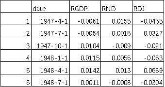
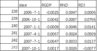
then aggregate the date list and three log growth rates into a data frame named “LogRtn”, then print the head and tail of the data frame. There are 243 rows of data from 1947Q2 to 2007Q4.
|
Head:
Tail:
|
(b) summary statistics of the three growth rate variables,
|
As shown above, the quarterly standard deviation of RDJ is the largest, which indicate the growth rate of Dow Jones Index are more volatile than RGDP and RND. |
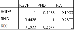
(c) the correlation matrix of RGDP, RND, RDJ is
|
Correlation between these three variables are all positive. |
(d) autocorrelations of RGDP, RND, RDJ, for 0 to 6 lags are listed as below
 |
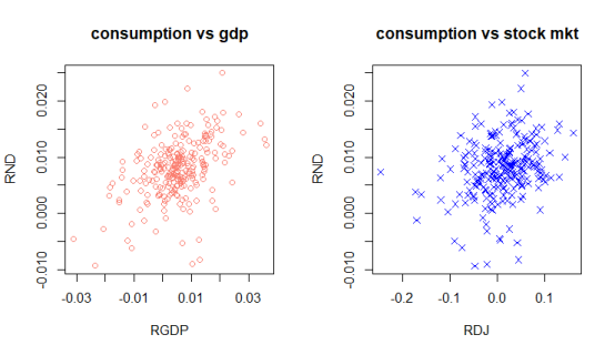
(e) scatterplot of real consumption growth against real income growth is shown on the left, and scatterplot of real consumption growth against real stock market growth is shown on the right.
 |
Question 2
We run OLS regression of consumption growth rate on explanatory variable
  , where
  and
and  the summary of three regressions are,
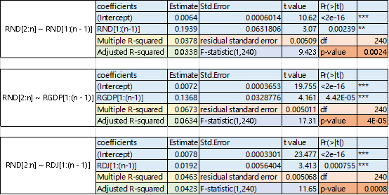
The infective of the regression equation together with the regression coefficients are distinctness by significance testing when significance level equals 0.05, because the coefficients’ p values are all less than 0.05, and the whole equation p-values are less than 0.05.
We must notice that three Multiple R-squared are too small, less than 10%, which means the explanatory variables are not sufficient to predict the consumption growth rate.
we add the lag consumption growth and historical GDP growth rate and historical DJ growth rate into OLS equation, then we have the following result. the R-square is 0.0986, which tell us add more explanatory variables do much better in prediction. but the coefficient of  is not significant any more.

Then we add lags(lag=2) of consumption, income and stock market into OLS regression, then we get the following result.

Question 3
(a) the summary of GDP growth on lagged GDP growth( lags=4) are listed as below,

Then we change the explanatory variables with lagged consumption growth and stock market growth rate (RND, RDJ). The multiple R-squared become 26.7%, which indicate that the RND and RDJ can predict RGDP.

(b) after run the OLS regression of  , the coefficients
 . we plot the fitted values of
  as below on the left.
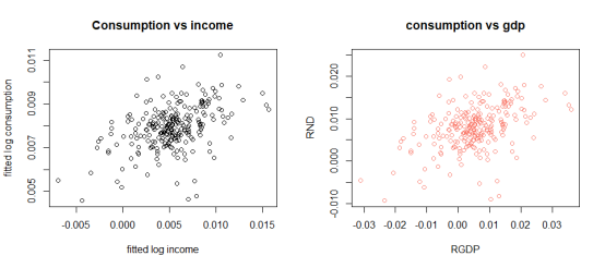
Compared with the scatterplot of original data of RND(consumption) and RGDP(income), we can find that the degree of dispersion in the left plot is smaller, when the shape is almost the same.
The correlation between the fitted values of consumption growth and income growth is 0.44.
(c) in R package “AER”, we can use![]() command to conduct instrument variable regression.
command to conduct instrument variable regression.
Y<- RND[2:n] is dependent variable, Yhat<- fitted(Y) is endogenous variable,
X<-RGDP[1: (n-1)] is instrument, Xhat<-fitted(RGDP[2:n]) is instrument,
Run  , then we get the lambda = 0.136.
代写CS& Finance|建模|代码|系统|报告|考试
编程类: C++,JAVA ,数据库,WEB,Linux,Nodejs,JSP,Html,Prolog,Python,Haskell,hadoop算法,系统机器学习
金融类:统计,计量,风险投资,金融工程,R语言,Python语言,Matlab,建立模型,数据分析,数据处理
服务类: Lab/Assignment/Project/Course/Qzui/Midterm/Final/Exam/Test帮助代写代考辅导
天才写手 , 代写CS , 代写finance , 代写statistics , 考试助攻
E-mail:[email protected] 微信:BadGeniuscs 工作时间:无休息工作日-早上8点到凌晨3点
如果您用的手机请先保存二维码到手机里面,识别图中二维码。如果用电脑,直接掏出手机果断扫描。

