F79MA 2018-19: Assessed Project 1 Report
Introduction and Summary
This project is aim to look at parameter estimation for an inverse gamma model, which can be considered as a survival distribution. Also, we will show that computer simulation can be a very useful tool to characterize the performance of statistical estimators.

Analysis
The probability density function of inverse distribution is

where ![]() is a shape parameter,
is a shape parameter, ![]() is a scale parameter, and
is a scale parameter, and ![]() is the gamma function.
is the gamma function.
Let ![]() be a random sample from an inverse gamma distribution with shape parameter
be a random sample from an inverse gamma distribution with shape parameter ![]() and unknown scale parameter
and unknown scale parameter ![]() .
.
Task 1
As ![]() is i.i.d, the joint density function is
is i.i.d, the joint density function is

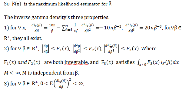
Then

Differentiating with respect to ![]() , we get the likelihood equation
, we get the likelihood equation

Differentiating again, we get

Which is negative for all ![]() , and any n.
, and any n.
Solving equation (1.3) for ![]() , we get
, we get


因部分公式不兼容请查看doc文档
r code:
rm(list=ls(all=TRUE))
library('invgamma')

# task 3
alpha<-10
beta<-1   #true value

ntime<-1000
nmax<-50
betahat<-rep(0,ntime)
vac<-rep(0,nmax)
MSE<-rep(0,nmax)

for (n in 1:nmax){
  # repeat times
  for (t in 1:ntime){
    Y<-rinvgamma(n,alpha,rate=1)
    betahat[t]<-alpha/mean(1/Y)
  }
  vac[n]<-var(betahat)
  MSE[n]<-1/ntime*sum(betahat-beta)^2
}

n<-c(1:50)
plot(n,MSE,main='MSE vs n')


# task 5
crbound<-beta^2/alpha/n^2
plot(MSE-crbound)
abline(h=0,col='red')

# task 6
betas<-c(0.3,0.5,0.8,1,1.2)
MSEMME<-matrix(0,nrow=5,ncol=3)
MSEMLE<-matrix(0,nrow=5,ncol=3)
ns<-c(20,40,60)

for (i in 1:5){
  beta<-betas[i]
  for (j in 1:3){
    n<-ns[j]
    mme<-rep(0,100)
    mle<-rep(0,100)
    for (t in 1:100){
      sp<- rinvgamma(n,alpha,beta)
      mme[t]<-mean(sp)*((mean(sp))^2/var(sp)+1)
      mle[t]<-alpha/mean(1/sp)
    }
    MSEMME[i,j]<-1/100*sum((mme-beta)^2)
    MSEMLE[i,j]<-1/100*sum((mle-beta)^2)
  }
}

round(MSEMME,4)
round(MSEMLE,4)

# task 7
betas<-c(0.3,0.5,0.8,1,1.2)
AVsMLE<-matrix(0,nrow=5,ncol=3)
ns<-c(20,40,60)

for (i in 1:5){
  beta<-betas[i]
  for (j in 1:3){
    n<-ns[j]
    mle<-rep(0,100)
    for (t in 1:100){
      sp<- rinvgamma(n,alpha,beta)
      mle[t]<-alpha/mean(1/sp)
    }
    AVsMLE[i,j]<-sd(mle)
  }
}
round(AVsMLE,4)
最先出自天才代写 数据库代写
合作:幽灵代写
