Course Project Part III – 60pts
DATE START / END ‘2014-06-01’, ‘2016-06-13’
Part III – Correlation and Panda – 60 pts
In this part, we will configure the airline industry stock.
|
#1 |
American Airlines Group Inc. |
AAL |
||
|
#2 |
Alaska Air Group, Inc. |
ALK |
||
|
#3 |
Avianca Holdings S.A. |
AVH |
||
|
#4 |
China Eastern Airlines Corporation Ltd. CEA |
|||
|
#5 |
China Southern Airlines Company Limited ZNH |
|||
|
#6 |
Controladora Vuela Compania de Aviacion, S.A.B. de C.V. VLRS |
|||
|
#7 |
Copa Holdings, S.A. |
CPA |
||
|
#8 |
Delta Air Lines, Inc. |
DAL |
||
|
#9 |
Gol Linhas Aereas Inteligentes S.A. GOL |
|||
|
#10 |
LATAM Airlines Group S.A. LFL |
|||
|
#11 |
Southwest Airlines Company |
LUV |
||
|
#12 |
United Continental Holdings, Inc. |
UAL |
||
# 13 You will use WTI as an information about the CRUDE OIL PRICE
Task 1 (5pts)

You will not load the information from Southwest the same way.
It will be stored into a dictionary indexed by the name of the symbols.
It will represented by this following dictionary.
all_data[LIST_OF_SYMBOLS]
example: all_data[“LFL”]
>>> print (all_data[‘AAL’].head(2))
Open High Low Close Volume Adj Close
Date
2014-06-02 40.000000 41.25 40.000000 41.220001 9902100 40.213663
2014-06-03 41.130001 42.09 41.110001 41.439999 9456200 40.428290
1
Task 2 (5pts)
Load the market data from Southwest Airlines from the CSV file ‘LUV.csv’.
Store this data into the variable luvdf.
The problem of reading a csv file is that your dates have a string type. You need to cast this string into a DateIndex for the dataframe you will be using in the rest of your code.
print(luvdf.head(2))
Open High Low Close Volume Adj Close
Date
2014-05-01 19.18 19.219999 18.450001 18.580000 603800 18.123725
2014-05-02 18.66 19.299999 18.629999 18.969999 556600 18.504147
Hint: read_csv from the panda library has different options that you can use to cast a date (string type) to a dateindex. I am suggesting you to check the argument of this function: parses_date and index_col.
Task 3 (5pts)
As you certainly noticed, the starting date of luvdf is different from the starting date of the other symbols.
In this task you will add a key to the dictionary all_data that you will call ‘LUV’ and you will assign the dates of luvf corresponding to the same interval as the other symbols.
Hint: you will need to use: luvdf[‘DATESTART’:’DATEEND’]
Task 4 (5pts)
You create a dataframe price containing only the prices “Adj Close” of all the symbols.
… print(price.head(2))
AAL ALK AVH CEA CPA DAL \
Date
2014-06-02 40.213663 48.630584 14.395138 15.058780 130.267298
39.719238
2014-06-03 40.428290 48.543110 14.227547 15.078451 129.974899
40.089445
GOL LFL LUV UAL VLRS WTI ZNH
Date
2014-06-02 56.200002 14.16 14.073248 46.700001 8.57 14.073248 13.883791
2014-06-03 55.700002 14.19 13.955398 47.509998 8.43 13.955398 14.093573
2
You create a dataframe volume containing only the volume of all the symbols.
Task 5 (5pts)
Using the function pct_change(), you will calculate the daily return for each of the symbols. You will store the results into the variable daily_return. This return will be calculated out of the Adj Price.
Now without using pct_change(), you will use shift(1), you will calculate the daily return. You will compare these results with the the results returning by pct_change.
Task 6 (5pts)
Create the scatter plot between the return of AAL and the Volume. Do you see any correlation?
Create the scatter plot between the return of LUV and the Volume. Do you see any correlation?
Task 7 (5pts)
Print the pair-correlation between all the symbols.
You will also print a graphic between the correlation of all the symbols:
pd.scatter_matrix(DataFrameToSpecify, diagonal=‘kde’, figsize=(10, 10));
Task 8 (5pts)
Using the function rolling_mean from panda, calculate the rolling average for 5 days of all the symbols. You will store this new column into the all_data[SYMBOL]. This symbol will be called MovingAverage.
Task 9 (5pts)
You will need to get rid of the symbol WTI being the crude oil.
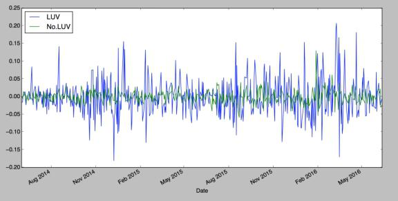
Let’s create a DataFrame noluv containing the mean of the return of all the symbols excep LUV for each day. You will need to use the command drop(‘LUV’) to remove LUV which will not be a part of the moving average.
Let’s create a second DataFrame onlyluv containing the return of LUV.
Create another dataframe containing the aggregation of noluv and onlyluv.
You will use this command.
tt=pd.DataFrame({‘No.LUV’ : noluv , ‘LUV’ : onlyluv})
You will plot the daily return for the whole period.
tt.plot()


With this chart, it is not possible to say anything.
Try to make appear a trend between the movement of LUV and the rest of the Airline industry.
Use different value of the moving average to see if you can have a clearer way of seeing the relation between LUV and the rest of the Airline industry.
Hint: you can just use moving average associated to the
pd.rolling_mean(tt,X).plot()
Replace X by the value you prefer. [you may find a lag of LUV].
Task 10 (5pts)
Draw the graphic representing the expected returns with the risk.
Expected returns being the mean of the daily return and the risk being the standard deviation of the daily returns.
You will use daily_return.mean() for the expected return and daily_return.std() for the risk.
Task 11 (10pts)
You will study the correlation between the average return of the airline industry with the price of crude oil WTI.
a) plot the scatter plot of the average of the daily return of the whole airline industry and the price of the Adjusted Close of WTI.
b) plot the scatter plot of the average of the daily return of the whole airline industry and the daily return of the Adjusted Close of WTI.
c) using the function lm = smf.ols(formula=“????”, data=…).fit()
Find the parameter of the linear regression
d) plot the least square line
![]()
